2.5. Dynamics

There are now different rheologies available in the CICE code. The elastic-viscous-plastic (EVP) model represents a modification of the standard viscous-plastic (VP) model for sea ice dynamics [11]. The elastic-anisotropic-plastic (EAP) model, on the other hand, explicitly accounts for the observed sub-continuum anisotropy of the sea ice cover [53][51]. If kdyn = 1 in the namelist then the EVP rheology is used (module ice_dyn_evp.F90), while kdyn = 2 is associated with the EAP rheology (ice_dyn_eap.F90). At times scales associated with the wind forcing, the EVP model reduces to the VP model while the EAP model reduces to the anisotropic rheology described in detail in [53][48]. At shorter time scales the adjustment process takes place in both models by a numerically more efficient elastic wave mechanism. While retaining the essential physics, this elastic wave modification leads to a fully explicit numerical scheme which greatly improves the model’s computational efficiency.

The EVP sea ice dynamics model is thoroughly documented in [17], [16], [18] and [19] and the EAP dynamics in [48]. Simulation results and performance of the EVP and EAP models have been compared with the VP model and with each other in realistic simulations of the Arctic respectively in [21] and [48]. Here we summarize the equations and direct the reader to the above references for details. The numerical implementation in this code release is that of [18] and [19], with revisions to the numerical solver as in [4]. The implementation of the EAP sea ice dynamics into CICE is described in detail in [48].

2.5.1. Momentum

The force balance per unit area in the ice pack is given by a two-dimensional momentum equation [11], obtained by integrating the 3D equation through the thickness of the ice in the vertical direction:

(1)\[m{\partial {\bf u}\over\partial t} = \nabla\cdot{\bf \sigma} + \vec{\tau}_a+\vec{\tau}_w + \vec{\tau}_b - \hat{k}\times mf{\bf u} - mg\nabla H_\circ,\]

where \(m\) is the combined mass of ice and snow per unit area and \(\vec{\tau}_a\) and \(\vec{\tau}_w\) are wind and ocean stresses, respectively. The term \(\vec{\tau}_b\) is a seabed stress (also referred to as basal stress) that represents the grounding of pressure ridges in shallow water [26]. The mechanical properties of the ice are represented by the internal stress tensor \(\sigma_{ij}\). The other two terms on the right hand side are stresses due to Coriolis effects and the sea surface slope. The parameterization for the wind and ice–ocean stress terms must contain the ice concentration as a multiplicative factor to be consistent with the formal theory of free drift in low ice concentration regions. A careful explanation of the issue and its continuum solution is provided in [19] and [5].

The momentum equation is discretized in time as follows, for the classic EVP approach. First, for clarity, the two components of Equation (1) are

\[\begin{split}\begin{aligned} m{\partial u\over\partial t} &=& {\partial\sigma_{1j}\over\partial x_j} + \tau_{ax} + a_i c_w \rho_w \left|{\bf U}_w - {\bf u}\right| \left[\left(U_w-u\right)\cos\theta - \left(V_w-v\right)\sin\theta\right] -C_bu +mfv - mg{\partial H_\circ\over\partial x}, \\ m{\partial v\over\partial t} &=& {\partial\sigma_{2j}\over\partial x_j} + \tau_{ay} + a_i c_w \rho_w \left|{\bf U}_w - {\bf u}\right| \left[\left(U_w-u\right)\sin\theta + \left(V_w-v\right)\cos\theta\right] -C_bv-mfu - mg{\partial H_\circ\over\partial y}. \end{aligned}\end{split}\]

In the code, \({\tt vrel}=a_i c_w \rho_w\left|{\bf U}_w - {\bf u}^k\right|\) and \(C_b=T_b \left( \sqrt{(u^k)^2+(v^k)^2}+u_0 \right)^{-1}\), where \(k\) denotes the subcycling step. The following equations illustrate the time discretization and define some of the other variables used in the code.

(2)\[\underbrace{\left({m\over\Delta t_e}+{\tt vrel} \cos\theta\ + C_b \right)}_{\tt cca} u^{k+1} - \underbrace{\left(mf+{\tt vrel}\sin\theta\right)}_{\tt ccb}v^{k+1} = \underbrace{{\partial\sigma_{1j}^{k+1}\over\partial x_j}}_{\tt strintx} + \underbrace{\tau_{ax} - mg{\partial H_\circ\over\partial x} }_{\tt forcex} + {\tt vrel}\underbrace{\left(U_w\cos\theta-V_w\sin\theta\right)}_{\tt waterx} + {m\over\Delta t_e}u^k,\]

(3)\[\underbrace{\left(mf+{\tt vrel}\sin\theta\right)}_{\tt ccb} u^{k+1} + \underbrace{\left({m\over\Delta t_e}+{\tt vrel} \cos\theta + C_b \right)}_{\tt cca}v^{k+1} = \underbrace{{\partial\sigma_{2j}^{k+1}\over\partial x_j}}_{\tt strinty} + \underbrace{\tau_{ay} - mg{\partial H_\circ\over\partial y} }_{\tt forcey} + {\tt vrel}\underbrace{\left(U_w\sin\theta+V_w\cos\theta\right)}_{\tt watery} + {m\over\Delta t_e}v^k,\]

and vrel\(\cdot\)waterx(y) = taux(y).

We solve this system of equations analytically for \(u^{k+1}\) and \(v^{k+1}\). Define

(4)\[\hat{u} = F_u + \tau_{ax} - mg{\partial H_\circ\over\partial x} + {\tt vrel} \left(U_w\cos\theta - V_w\sin\theta\right) + {m\over\Delta t_e}u^k\]

(5)\[\hat{v} = F_v + \tau_{ay} - mg{\partial H_\circ\over\partial y} + {\tt vrel} \left(U_w\sin\theta + V_w\cos\theta\right) + {m\over\Delta t_e}v^k,\]

where \({\bf F} = \nabla\cdot\sigma^{k+1}\). Then

\[\begin{split}\begin{aligned} \left({m\over\Delta t_e} +{\tt vrel}\cos\theta\ + C_b \right)u^{k+1} - \left(mf + {\tt vrel}\sin\theta\right) v^{k+1} &=& \hat{u} \\ \left(mf + {\tt vrel}\sin\theta\right) u^{k+1} + \left({m\over\Delta t_e} +{\tt vrel}\cos\theta + C_b \right)v^{k+1} &=& \hat{v}.\end{aligned}\end{split}\]

Solving simultaneously for \(u^{k+1}\) and \(v^{k+1}\),

\[\begin{split}\begin{aligned} u^{k+1} = {a \hat{u} + b \hat{v} \over a^2 + b^2} \\ v^{k+1} = {a \hat{v} - b \hat{u} \over a^2 + b^2}, \end{aligned}\end{split}\]

where

(6)\[\begin{split}a = {m\over\Delta t_e} + {\tt vrel}\cos\theta + C_b \\\end{split}\]

(7)\[b = mf + {\tt vrel}\sin\theta.\]

When the subcycling is finished for each (thermodynamic) time step, the ice–ocean stress must be constructed from taux(y) and the terms containing vrel on the left hand side of the equations.

The Hibler-Bryan form for the ice-ocean stress [13] is included in ice_dyn_shared.F90 but is currently commented out, pending further testing.

2.5.2. Seabed stress

The parameterization for the seabed stress is described in [26]. The components of the basal seabed stress are \(\tau_{bx}=C_bu\) and \(\tau_{by}=C_bv\), where \(C_b\) is a coefficient expressed as

(8)\[\begin{split}C_b= k_2 \max [0,(h_u - h_{cu})] e^{-\alpha_b * (1 - a_u)} (\sqrt{u^2+v^2}+u_0)^{-1}, \\\end{split}\]

where \(k_2\) determines the maximum seabed stress that can be sustained by the grounded parameterized ridge(s), \(u_0\) is a small residual velocity and \(\alpha_b=20\) is a parameter to ensure that the seabed stress quickly drops when the ice concentration is smaller than 1. In the code, \(k_2 \max [0,(h_u - h_{cu})] e^{-\alpha_b * (1 - a_u)}\) is defined as \(T_b\). The quantities \(h_u\), \(a_{u}\) and \(h_{cu}\) are calculated at the ‘u’ point based on local ice conditions (surrounding tracer points). They are respectively given by

(9)\[\begin{split}h_u=\max[v_i(i,j),v_i(i+1,j),v_i(i,j+1),v_i(i+1,j+1)], \\\end{split}\]

(10)\[\begin{split}a_u=\max[a_i(i,j),a_i(i+1,j),a_i(i,j+1),a_i(i+1,j+1)]. \\\end{split}\]

(11)\[\begin{split}h_{cu}=a_u h_{wu} / k_1, \\\end{split}\]

where the \(a_i\) and \(v_i\) are the total ice concentrations and ice volumes around the \(u\) point \(i,j\) and \(k_1\) is a parameter that defines the critical ice thickness \(h_{cu}\) at which the parameterized ridge(s) reaches the seafloor for a water depth \(h_{wu}=\min[h_w(i,j),h_w(i+1,j),h_w(i,j+1),h_w(i+1,j+1)]\). Given the formulation of \(C_b\) in equation (8), the seabed stress components are non-zero only when \(h_u > h_{cu}\).

The maximum seabed stress depends on the weigth of the ridge above hydrostatic balance and the value of \(k_2\). It is, however, the parameter \(k_1\) that has the most notable impact on the simulated extent of landfast ice. The value of \(k_1\) can be changed at runtime using the namelist variable k1. The grounding scheme can be turned on or off using the namelist logical basalstress.

Note that the user must provide a bathymetry field for using this grounding scheme. It is suggested to have a bathymetry field with water depths larger than 5 m that represents well shallow water regions such as the Laptev Sea and the East Siberian Sea. To prevent unrealistic grounding, \(T_b\) is set to zero when \(h_{wu}\) is larger than 30 m. This maximum value is chosen based on observations of large keels in the Arctic Ocean [1].

2.5.3. Internal stress

For convenience we formulate the stress tensor \(\bf \sigma\) in terms of \(\sigma_1=\sigma_{11}+\sigma_{22}\), \(\sigma_2=\sigma_{11}-\sigma_{22}\), and introduce the divergence, \(D_D\), and the horizontal tension and shearing strain rates, \(D_T\) and \(D_S\) respectively.

CICE now outputs the internal ice pressure which is an important field to support navigation in ice-infested water. The internal ice pressure \((sigP)\) is the average of the normal stresses multiplied by \(-1\) and is therefore simply equal to \(-\sigma_1/2\).

Elastic-Viscous-Plastic

In the EVP model the internal stress tensor is determined from a regularized version of the VP constitutive law. Following the approach of [2] (see also [26]), the elliptical yield curve can be modified such that the ice has isotropic tensile strength. The tensile strength \(T_p\) is expressed as a fraction of the ice strength \(P\), that is \(T_p=k_t P\) where \(k_t\) should be set to a value between 0 and 1 (this can be changed at runtime with the namelist parameter Ktens). The constitutive law is therefore

(12)\[\begin{split}{1\over E}{\partial\sigma_1\over\partial t} + {\sigma_1\over 2\zeta} + {P_R(1-k_t)\over 2\zeta} = D_D, \\\end{split}\]

(13)\[{1\over E}{\partial\sigma_2\over\partial t} + {\sigma_2\over 2\eta} = D_T,\]

(14)\[{1\over E}{\partial\sigma_{12}\over\partial t} + {\sigma_{12}\over 2\eta} = {1\over 2}D_S,\]

where

\[D_D = \dot{\epsilon}_{11} + \dot{\epsilon}_{22},\]

\[D_T = \dot{\epsilon}_{11} - \dot{\epsilon}_{22},\]

\[D_S = 2\dot{\epsilon}_{12},\]

\[\dot{\epsilon}_{ij} = {1\over 2}\left({{\partial u_i}\over{\partial x_j}} + {{\partial u_j}\over{\partial x_i}}\right),\]

\[\zeta = {P(1+k_t)\over 2\Delta},\]

\[\eta = {P(1+k_t)\over {2\Delta e^2}},\]

\[\Delta = \left[D_D^2 + {1\over e^2}\left(D_T^2 + D_S^2\right)\right]^{1/2},\]

and \(P_R\) is a “replacement pressure” (see [9], for example), which serves to prevent residual ice motion due to spatial variations of \(P\) when the rates of strain are exactly zero. The ice strength \(P\) is a function of the ice thickness and concentration as it is described in the Icepack Documentation. The parameteter \(e\) is the ratio of the major and minor axes of the elliptical yield curve, also called the ellipse aspect ratio. It can be changed using the namelist parameter e_ratio.

Viscosities are updated during the subcycling, so that the entire dynamics component is subcycled within the time step, and the elastic parameter \(E\) is defined in terms of a damping timescale \(T\) for elastic waves, \(\Delta t_e < T < \Delta t\), as

\[E = {\zeta\over T},\]

where \(T=E_\circ\Delta t\) and \(E_\circ\) (eyc) is a tunable parameter less than one. Including the modification proposed by [4] for equations (13) and (14) in order to improve numerical convergence, the stress equations become

\[\begin{split}\begin{aligned} {\partial\sigma_1\over\partial t} + {\sigma_1\over 2T} + {P_R(1-k_t)\over 2T} &=& {P(1+k_t)\over 2T\Delta} D_D, \\ {\partial\sigma_2\over\partial t} + {\sigma_2\over 2T} &=& {P(1+k_t)\over 2Te^2\Delta} D_T,\\ {\partial\sigma_{12}\over\partial t} + {\sigma_{12}\over 2T} &=& {P(1+k_t)\over 4Te^2\Delta}D_S.\end{aligned}\end{split}\]

Once discretized in time, these last three equations are written as

(15)\[\begin{split}\begin{aligned} {(\sigma_1^{k+1}-\sigma_1^{k})\over\Delta t_e} + {\sigma_1^{k+1}\over 2T} + {P_R^k(1-k_t)\over 2T} &=& {P(1+k_t)\over 2T\Delta^k} D_D^k, \\ {(\sigma_2^{k+1}-\sigma_2^{k})\over\Delta t_e} + {\sigma_2^{k+1}\over 2T} &=& {P(1+k_t)\over 2Te^2\Delta^k} D_T^k,\\ {(\sigma_{12}^{k+1}-\sigma_{12}^{k})\over\Delta t_e} + {\sigma_{12}^{k+1}\over 2T} &=& {P(1+k_t)\over 4Te^2\Delta^k}D_S^k,\end{aligned}\end{split}\]

where \(k\) denotes again the subcycling step. All coefficients on the left-hand side are constant except for \(P_R\). This modification compensates for the decreased efficiency of including the viscosity terms in the subcycling. (Note that the viscosities do not appear explicitly.) Choices of the parameters used to define \(E\), \(T\) and \(\Delta t_e\) are discussed in Sections Revised approach and Choosing an appropriate time step.

The bilinear discretization used for the stress terms \(\partial\sigma_{ij}/\partial x_j\) in the momentum equation is now used, which enabled the discrete equations to be derived from the continuous equations written in curvilinear coordinates. In this manner, metric terms associated with the curvature of the grid are incorporated into the discretization explicitly. Details pertaining to the spatial discretization are found in [18].

Elastic-Anisotropic-Plastic

In the EAP model the internal stress tensor is related to the geometrical properties and orientation of underlying virtual diamond shaped floes (see Diamond-shaped floes). In contrast to the isotropic EVP rheology, the anisotropic plastic yield curve within the EAP rheology depends on the relative orientation of the diamond shaped floes (unit vector \(\mathbf r\) in Diamond-shaped floes), with respect to the principal direction of the deformation rate (not shown). Local anisotropy of the sea ice cover is accounted for by an additional prognostic variable, the structure tensor \(\mathbf{A}\) defined by

\[{\mathbf A}=\int_{\mathbb{S}}\vartheta(\mathbf r)\mathbf r\mathbf r d\mathbf r\label{structuretensor}.\]

where \(\mathbb{S}\) is a unit-radius circle; A is a unit trace, 2\(\times\)2 matrix. From now on we shall describe the orientational distribution of floes using the structure tensor. For simplicity we take the probability density function \(\vartheta(\mathbf r )\) to be Gaussian, \(\vartheta(z)=\omega_{1}\exp(-\omega_{2}z^{2})\), where \(z\) is the ice floe inclination with respect to the axis \(x_{1}\) of preferential alignment of ice floes (see Diamond-shaped floes), \(\vartheta(z)\) is periodic with period \(\pi\), and the positive coefficients \(\omega_{1}\) and \(\omega_{2}\) are calculated to ensure normalization of \(\vartheta(z)\), i.e. \(\int_{0}^{2\pi}\vartheta(z)dz=1\). The ratio of the principal components of \(\mathbf{A}\), \(A_{1}/A_{2}\), are derived from the phenomenological evolution equation for the structure tensor \(\mathbf A\),

(16)\[\frac{D\mathbf{A}}{D t}=\mathbf{F}_{iso}(\mathbf{A})+\mathbf{F}_{frac}(\mathbf{A},\boldsymbol\sigma),\]

where \(t\) is the time, and \(D/Dt\) is the co-rotational time derivative accounting for advection and rigid body rotation (\(D\mathbf A/Dt = d\mathbf A/dt -\mathbf W \cdot \mathbf A -\mathbf A \cdot \mathbf W^{T}\)) with \(\mathbf W\) being the vorticity tensor. \(\mathbf F_{iso}\) is a function that accounts for a variety of processes (thermal cracking, melting, freezing together of floes) that contribute to a more isotropic nature to the ice cover. \(\mathbf F_{frac}\) is a function determining the ice floe re-orientation due to fracture, and explicitly depends upon sea ice stress (but not its magnitude). Following [53], based on laboratory experiments by [43] we consider four failure mechanisms for the Arctic sea ice cover. These are determined by the ratio of the principal values of the sea ice stress \(\sigma_{1}\) and \(\sigma_{2}\): (i) under biaxial tension, fractures form across the perpendicular principal axes and therefore counteract any apparent redistribution of the floe orientation; (ii) if only one of the principal stresses is compressive, failure occurs through axial splitting along the compression direction; (iii) under biaxial compression with a low confinement ratio, (\(\sigma_{1}/\sigma_{2}<R\)), sea ice fails Coulombically through formation of slip lines delineating new ice floes oriented along the largest compressive stress; and finally (iv) under biaxial compression with a large confinement ratio, (\(\sigma_{1}/\sigma_{2}\ge R\)), the ice is expected to fail along both principal directions so that the cumulative directional effect balances to zero.

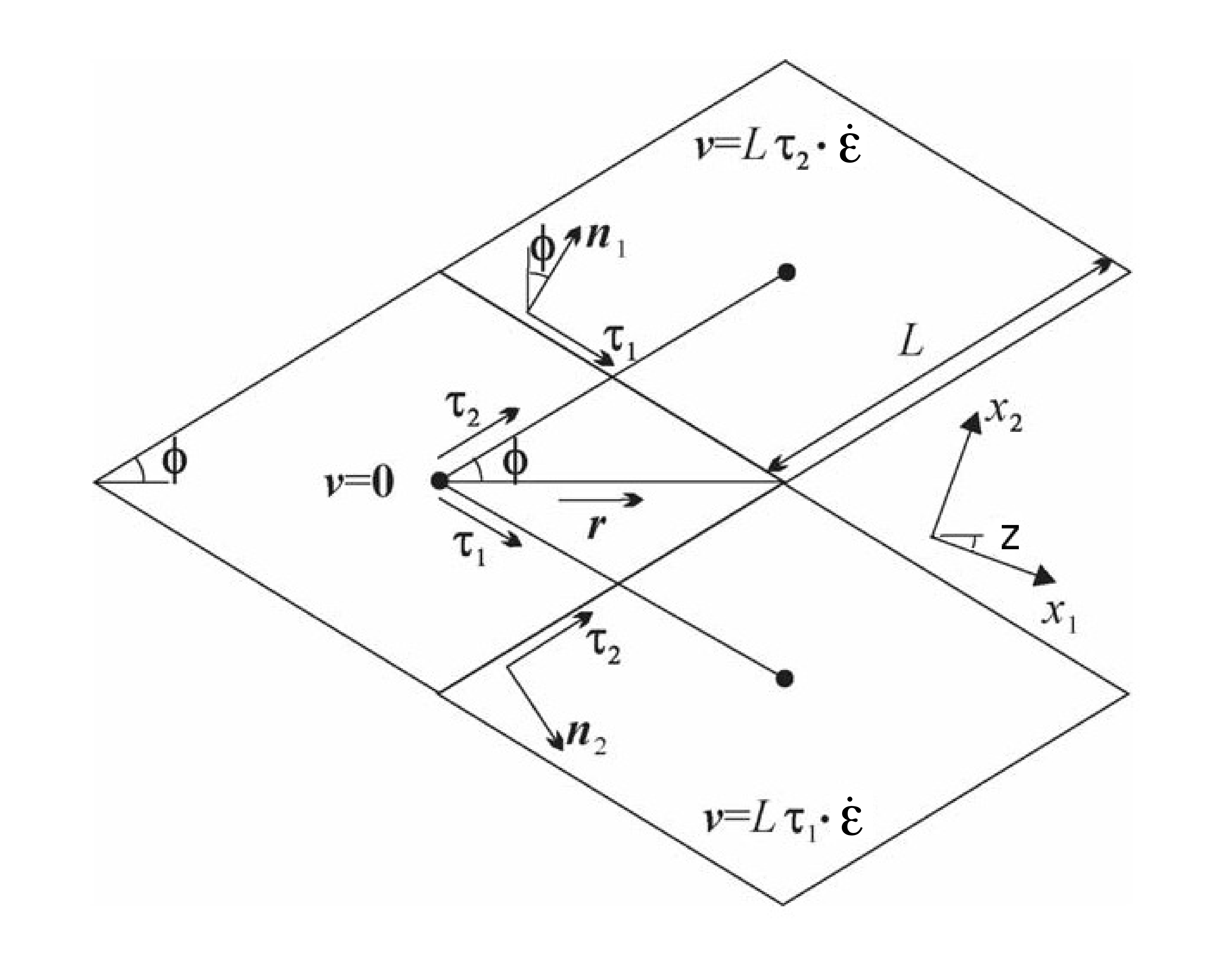
Diamond-shaped floes

Figure Diamond-shaped floes shows geometry of interlocking diamond-shaped floes (taken from [53]). \(\phi\) is half of the acute angle of the diamonds. \(L\) is the edge length. \(\boldsymbol n_{1}\), \(\boldsymbol n_{2}\) and \(\boldsymbol\tau_{1}\), \(\boldsymbol\tau_{2}\) are respectively the normal and tangential unit vectors along the diamond edges. \(\mathbf v=L\boldsymbol\tau_{2}\cdot\dot{\boldsymbol\epsilon}\) is the relative velocity between the two floes connected by the vector \(L \boldsymbol \tau_{2}\). \(\mathbf r\) is the unit vector along the main diagonal of the diamond. Note that the diamonds illustrated here represent one possible realisation of all possible orientations. The angle \(z\) represents the rotation of the diamonds’ main axis relative to their preferential orientation along the axis \(x_1\).

The new anisotropic rheology requires solving the evolution Equation (16) for the structure tensor in addition to the momentum and stress equations. The evolution equation for \(\mathbf{A}\) is solved within the EVP subcycling loop, and consistently with the momentum and stress evolution equations, we neglect the advection term for the structure tensor. Equation (16) then reduces to the system of two equations:

\[\begin{split}\begin{aligned} \frac{\partial A_{11}}{\partial t}&=&-k_{t}\left(A_{11}-\frac{1}{2}\right)+M_{11} \mbox{,} \\ \frac{\partial A_{12}}{\partial t}&=&-k_{t} A_{12}+M_{12} \mbox{,}\end{aligned}\end{split}\]

where the first terms on the right hand side correspond to the isotropic contribution, \(F_{iso}\), and \(M_{11}\) and \(M_{12}\) are the components of the term \(F_{frac}\) in Equation (16) that are given in [53] and [48]. These evolution equations are discretized semi-implicitly in time. The degree of anisotropy is measured by the largest eigenvalue (\(A_{1}\)) of this tensor (\(A_{2}=1-A_{1}\)). \(A_{1}=1\) corresponds to perfectly aligned floes and \(A_{1}=0.5\) to a uniform distribution of floe orientation. Note that while we have specified the aspect ratio of the diamond floes, through prescribing \(\phi\), we make no assumption about the size of the diamonds so that formally the theory is scale invariant.

As described in greater detail in [53], the internal ice stress for a single orientation of the ice floes can be calculated explicitly and decomposed, for an average ice thickness \(h\), into its ridging (r) and sliding (s) contributions

(17)\[\boldsymbol \sigma^{b}(\mathbf r,h)=P_{r}(h) \boldsymbol \sigma_{r}^{b}(\mathbf r)+P_{s}(h) \boldsymbol \sigma_{s}^{b}(\mathbf r),\]

where \(P_{r}\) and \(P_{s}\) are the ridging and sliding strengths and the ridging and sliding stresses are functions of the angle \(\theta= \arctan(\dot\epsilon_{II}/\dot\epsilon_{I})\), the angle \(y\) between the major principal axis of the strain rate tensor (not shown) and the structure tensor (\(x_1\) axis in Diamond-shaped floes, and the angle \(z\) defined in Diamond-shaped floes. In the stress expressions above the underlying floes are assumed parallel, but in a continuum-scale sea ice region the floes can possess different orientations in different places and we take the mean sea ice stress over a collection of floes to be given by the average

(18)\[\boldsymbol\sigma^{EAP}(h)=P_{r}(h)\int_{\mathbb{S}}\vartheta(\mathbf r)\left[\boldsymbol\sigma_{r}^{b}(\mathbf r)+ k \boldsymbol\sigma_{s}^{b}(\mathbf r)\right]d\mathbf r\]

where we have introduced the friction parameter \(k=P_{s}/P_{r}\) and where we identify the ridging ice strength \(P_{r}(h)\) with the strength \(P\) described in section 1 and used within the EVP framework.

As is the case for the EVP rheology, elasticity is included in the EAP description not to describe any physical effect, but to make use of the efficient, explicit numerical algorithm used to solve the full sea ice momentum balance. We use the analogous EAP stress equations,

(19)\[\frac{\partial \sigma_{1}}{\partial t}+\frac{\sigma_1}{2T} = \frac{\sigma^{EAP}_{1}}{2T} \mbox{,}\]

(20)\[\frac{\partial \sigma_{2}}{\partial t}+\frac{\sigma_2}{2T} = \frac{\sigma^{EAP}_{2}}{2T} \mbox{,}\]

(21)\[\frac{\partial \sigma_{12}}{\partial t}+\frac{\sigma_{12}}{2T} = \frac{\sigma^{EAP}_{12}}{2T} \mbox{,}\]

where the anisotropic stress \(\boldsymbol\sigma^{EAP}\) is defined in a look-up table for the current values of strain rate and structure tensor. The look-up table is constructed by computing the stress (normalized by the strength) from Equations (19)–(21) for discrete values of the largest eigenvalue of the structure tensor, \(\frac{1}{2}\le A_{1}\le 1\), the angle \(0\le\theta\le2\pi\), and the angle \(-\pi/2\le y\le\pi/2\) between the major principal axis of the strain rate tensor and the structure tensor [48]. The updated stress, after the elastic relaxation, is then passed to the momentum equation and the sea ice velocities are updated in the usual manner within the subcycling loop of the EVP rheology. The structure tensor evolution equations are solved implicitly at the same frequency, \(\Delta t_{e}\), as the ice velocities and internal stresses. Finally, to be coherent with our new rheology we compute the area loss rate due to ridging as \(\vert\dot{\boldsymbol\epsilon}\vert\alpha_{r}(\theta)\), with \(\alpha_r(\theta)\) and \(\alpha_s(\theta)\) given by [52],

\[\begin{aligned} \alpha_{r}(\theta)=\frac{\sigma^{r}_{ij}\dot\epsilon_{ij}}{P_{r} \vert\dot{\boldsymbol\epsilon}\vert } , \qquad \alpha_{s}(\theta)=\frac{\sigma^{s}_{ij}\dot\epsilon_{ij}}{P_{s} \vert\dot{\boldsymbol\epsilon}\vert }.\label{alphas}\end{aligned}\]

Both ridging rate and sea ice strength are computed in the outer loop of the dynamics.

2.5.4. Revised approach

The revised EVP approach is based on a pseudo-time iterative scheme [27], [4], [24]. By construction, the revised EVP approach should lead to the VP solution (given the right numerical parameters and a sufficiently large number of iterations). To do so, the inertial term is formulated such that it matches the backward Euler approach of implicit solvers and there is an additional term for the pseudo-time iteration. Hence, with the revised approach, the discretized momentum equations (2) and (3) become

(22)\[{\beta^*(u^{k+1}-u^k)\over\Delta t_e} + {m(u^{k+1}-u^n)\over\Delta t} + {\left({\tt vrel} \cos\theta + C_b \right)} u^{k+1} - {\left(mf+{\tt vrel}\sin\theta\right)} v^{k+1} = {{\partial\sigma_{1j}^{k+1}\over\partial x_j}} + {\tau_{ax} - mg{\partial H_\circ\over\partial x} } + {\tt vrel} {\left(U_w\cos\theta-V_w\sin\theta\right)},\]

(23)\[{\beta^*(v^{k+1}-v^k)\over\Delta t_e} + {m(v^{k+1}-v^n)\over\Delta t} + {\left({\tt vrel} \cos\theta + C_b \right)}v^{k+1} + {\left(mf+{\tt vrel}\sin\theta\right)} u^{k+1} = {{\partial\sigma_{2j}^{k+1}\over\partial x_j}} + {\tau_{ay} - mg{\partial H_\circ\over\partial y} } + {\tt vrel}{\left(U_w\sin\theta+V_w\cos\theta\right)},\]

where \(\beta^*\) is a numerical parameter and \(u^n, v^n\) are the components of the previous time level solution. With \(\beta=\beta^* \Delta t \left( m \Delta t_e \right)^{-1}\) [4], these equations can be written as

(24)\[\underbrace{\left((\beta+1){m\over\Delta t}+{\tt vrel} \cos\theta\ + C_b \right)}_{\tt cca} u^{k+1} - \underbrace{\left(mf+{\tt vrel}\sin\theta\right)}_{\tt ccb}v^{k+1} = \underbrace{{\partial\sigma_{1j}^{k+1}\over\partial x_j}}_{\tt strintx} + \underbrace{\tau_{ax} - mg{\partial H_\circ\over\partial x} }_{\tt forcex} + {\tt vrel}\underbrace{\left(U_w\cos\theta-V_w\sin\theta\right)}_{\tt waterx} + {m\over\Delta t}(\beta u^k + u^n),\]

(25)\[\underbrace{\left(mf+{\tt vrel}\sin\theta\right)}_{\tt ccb} u^{k+1} + \underbrace{\left((\beta+1){m\over\Delta t}+{\tt vrel} \cos\theta + C_b \right)}_{\tt cca}v^{k+1} = \underbrace{{\partial\sigma_{2j}^{k+1}\over\partial x_j}}_{\tt strinty} + \underbrace{\tau_{ay} - mg{\partial H_\circ\over\partial y} }_{\tt forcey} + {\tt vrel}\underbrace{\left(U_w\sin\theta+V_w\cos\theta\right)}_{\tt watery} + {m\over\Delta t}(\beta v^k + v^n),\]

At this point, the solutions \(u^{k+1}\) and \(v^{k+1}\) are obtained in the same manner as for the standard EVP approach (see equations (4) to (7)).

Introducing another numerical parameter \(\alpha=2T \Delta t_e ^{-1}\) [4], the stress equations in (15) become

\[\begin{split}\begin{aligned} {\alpha (\sigma_1^{k+1}-\sigma_1^{k})} + {\sigma_1^{k}} + {P_R^k(1-k_t)} &=& {P(1+k_t)\over \Delta^k} D_D^k, \\ {\alpha (\sigma_2^{k+1}-\sigma_2^{k})} + {\sigma_2^{k}} &=& {P(1+k_t)\over e^2\Delta^k} D_T^k,\\ {\alpha (\sigma_{12}^{k+1}-\sigma_{12}^{k})} + {\sigma_{12}^{k}} &=& {P(1+k_t)\over 2e^2\Delta^k}D_S^k,\end{aligned}\end{split}\]

where as opposed to the classic EVP, the second term in each equation is at iteration \(k\) [4]. Also, as opposed to the classic EVP, \(\Delta t_e\) times the number of subcycles (or iterations) does not need to be equal to the advective time step \(\Delta t\). Finally, as with the classic EVP approach, the stresses are initialized using the previous time level values. The revised EVP is activated by setting the namelist parameter revised_evp = true. In the code \(\alpha = arlx\) and \(\beta = brlx\). The values of \(arlx\) and \(brlx\) can be set in the namelist. It is recommended to use large values of these parameters and to set \(arlx=brlx\) [24].