2.4. Horizontal Transport

We wish to solve the continuity or transport equation (Equation (1)) for the fractional ice area in each thickness category \(n\). Equation (1) describes the conservation of ice area under horizontal transport. It is obtained from Equation (1) by discretizing \(g\) and neglecting the second and third terms on the right-hand side, which are treated separately (As described in the Icepack Documentation).

There are similar conservation equations for ice volume (Equation (2)), snow volume (Equation (3)), ice energy and snow energy:

(1)\[\frac{\partial e_{ink}}{\partial t} + \nabla \cdot (e_{ink} {\bf u}) = 0,\]

(2)\[\frac{\partial e_{snk}}{\partial t} + \nabla \cdot (e_{snk} {\bf u}) = 0.\]

By default, ice and snow are assumed to have constant densities, so that volume conservation is equivalent to mass conservation. Variable-density ice and snow layers can be transported conservatively by defining tracers corresponding to ice and snow density, as explained in the introductory comments in ice_transport_remap.F90. Prognostic equations for ice and/or snow density may be included in future model versions but have not yet been implemented.

Two transport schemes are available: upwind and the incremental remapping scheme of [7] as modified for sea ice by [30]. The remapping scheme has several desirable features:

• It conserves the quantity being transported (area, volume, or energy).

• It is non-oscillatory; that is, it does not create spurious ripples in the transported fields.

• It preserves tracer monotonicity. That is, it does not create new extrema in the thickness and enthalpy fields; the values at time \(m+1\) are bounded by the values at time \(m\).

• It is second-order accurate in space and therefore is much less diffusive than first-order schemes (e.g., upwind). The accuracy may be reduced locally to first order to preserve monotonicity.

• It is efficient for large numbers of categories or tracers. Much of the work is geometrical and is performed only once per grid cell instead of being repeated for each quantity being transported.

The time step is limited by the requirement that trajectories projected backward from grid cell corners are confined to the four surrounding cells; this is what is meant by incremental remapping as opposed to general remapping. This requirement leads to a CFL-like condition,

\[{\max|{\bf u}|\Delta t\over\Delta x} \leq 1.\]

For highly divergent velocity fields the maximum time step must be reduced by a factor of two to ensure that trajectories do not cross. However, ice velocity fields in climate models usually have small divergences per time step relative to the grid size.

The remapping algorithm can be summarized as follows:

1. Given mean values of the ice area and tracer fields in each grid cell, construct linear approximations of these fields. Limit the field gradients to preserve monotonicity.

2. Given ice velocities at grid cell corners, identify departure regions for the fluxes across each cell edge. Divide these departure regions into triangles and compute the coordinates of the triangle vertices.

3. Integrate the area and tracer fields over the departure triangles to obtain the area, volume, and energy transported across each cell edge.

4. Given these transports, update the state variables.

Since all scalar fields are transported by the same velocity field, step (2) is done only once per time step. The other three steps are repeated for each field in each thickness category. These steps are described below.

After the transport calculation, the sum of ice and open water areas within a grid cell may not add up to 1. The mechanical deformation parameterization in Icepack corrects this issue by ridging the ice and creating open water such that the ice and open water areas again add up to 1.

2.4.1. Reconstructing area and tracer fields

First, using the known values of the state variables, the ice area and tracer fields are reconstructed in each grid cell as linear functions of \(x\) and \(y\). For each field we compute the value at the cell center (i.e., at the origin of a 2D Cartesian coordinate system defined for that grid cell), along with gradients in the \(x\) and \(y\) directions. The gradients are limited to preserve monotonicity. When integrated over a grid cell, the reconstructed fields must have mean values equal to the known state variables, denoted by \(\bar{a}\) for fractional area, \(\tilde{h}\) for thickness, and \(\hat{q}\) for enthalpy. The mean values are not, in general, equal to the values at the cell center. For example, the mean ice area must equal the value at the centroid, which may not lie at the cell center.

Consider first the fractional ice area, the analog to fluid density \(\rho\) in [7]. For each thickness category we construct a field \(a({\bf r})\) whose mean is \(\bar{a}\), where \({\bf r} = (x,y)\) is the position vector relative to the cell center. That is, we require

(3)\[\int_A a \, dA = {\bar a} \, A,\]

where \(A=\int_A dA\) is the grid cell area. Equation (3) is satisfied if \(a({\bf r})\) has the form

(4)\[a({\bf r}) = \bar{a} + \alpha_a \left<\nabla a\right> \cdot ({\bf r}-{\bf \bar{r}}),\]

where \(\left<\nabla a\right>\) is a centered estimate of the area gradient within the cell, \(\alpha_a\) is a limiting coefficient that enforces monotonicity, and \({\bf \bar{r}}\) is the cell centroid:

\[{\bf \bar{r}} = {1\over A} \int_A {\bf r} \, dA.\]

It follows from Equation (4) that the ice area at the cell center (\(\mathbf{r} = 0\)) is

\[a_c = \bar{a} - a_x \overline{x} - a_y \overline{y},\]

where \(a_x = \alpha_a (\partial a / \partial x)\) and \(a_y = \alpha_a (\partial a / \partial y)\) are the limited gradients in the \(x\) and \(y\) directions, respectively, and the components of \({\bf \bar{r}}\), \(\overline{x} = \int_A x \, dA / A\) and \(\overline{y} = \int_A y \, dA / A\), are evaluated using the triangle integration formulas described in Section Integrating fields. These means, along with higher-order means such as \(\overline{x^2}\), \(\overline{xy}\), and \(\overline{y^2}\), are computed once and stored.

Next consider the ice and snow thickness and enthalpy fields. Thickness is analogous to the tracer concentration \(T\) in [7], but there is no analog in [7] to the enthalpy. The reconstructed ice or snow thickness \(h({\bf r})\) and enthalpy \(q(\mathbf{r})\) must satisfy

(5)\[\int_A a \, h \, dA = \bar{a} \, \tilde{h} \, A,\]

(6)\[\int_A a \, h \, q \, dA = \bar{a} \, \tilde{h} \, \hat{q} \, A,\]

where \(\tilde{h}=h(\tilde{\bf r})\) is the thickness at the center of ice area, and \(\hat{q}=q(\hat{\bf r})\) is the enthalpy at the center of ice or snow volume. Equations (5) and (6) are satisfied when \(h({\bf r})\) and \(q({\bf r})\) are given by

(7)\[h({\bf r}) = \tilde{h} + \alpha_h \left<\nabla h\right> \cdot ({\bf r}-{\bf \tilde{r}}),\]

(8)\[q({\bf r}) = \hat{q} + \alpha_q \left<\nabla q\right> \cdot ({\bf r}-{\bf \hat{r}}),\]

where \(\alpha_h\) and \(\alpha_q\) are limiting coefficients. The center of ice area, \({\bf\tilde{r}}\), and the center of ice or snow volume, \({\bf \hat{r}}\), are given by

\[{\bf \tilde{r}} = {1\over\bar{a} \, A}\int_A a \, {\bf r} \, dA,\]

\[{\bf \hat{r}} = {1\over\bar{a} \, \tilde{h} \, A}\int_A a \, h \, {\bf r} \, dA.\]

Evaluating the integrals, we find that the components of \({\bf \tilde{r}}\) are

\[\tilde{x} = \frac{a_c \overline{x}+a_x \overline{x^2}+a_y \overline{xy}} {\bar{a}},\]

\[\tilde{y} = \frac{a_c \overline{y}+a_x \overline{xy} +a_y \overline{y^2}} {\bar{a}},\]

and the components of \({\bf \hat{r}}\) are

\[\hat{x} = \frac { c_1 \overline{x} + c_2 \overline{x^2} + c_3 \overline{xy} + c_4 \overline{x^3} + c_5 \overline{x^2 y} + c_6 \overline{x y^2} } {\bar{a} \, \tilde{h}},\]

\[\hat{y} = \frac { c_1 \overline{y} + c_2 \overline{xy} + c_3 \overline{y^2} + c_4 \overline{x^2 y} + c_5 \overline{x y^2} + c_6 \overline{y^3} } {\bar{a} \, \tilde{h}},\]

where

\[\begin{split}\begin{aligned} c_1 & \equiv & a_c h_c, \\ c_2 & \equiv & a_c h_x + a_x h_c, \\ c_3 & \equiv & a_c h_y + a_y h_c, \\ c_4 & \equiv & a_x h_x, \\ c_5 & \equiv & a_x h_y + a_y h_x, \\ c_6 & \equiv & a_y h_y.\end{aligned}\end{split}\]

From Equation (7) and Equation (8), the thickness and enthalpy at the cell center are given by

\[h_c = \tilde{h} - h_x \tilde{x} - h_y \tilde{y},\]

\[q_c = \hat{q} - q_x \hat{x} - q_y \hat{y},\]

where \(h_x\), \(h_y\), \(q_x\) and \(q_y\) are the limited gradients of thickness and enthalpy. The surface temperature is treated the same way as ice or snow thickness, but it has no associated enthalpy. Tracers obeying conservation equations of the form Equation (7) and Equation (8) are treated in analogy to ice and snow enthalpy, respectively.

We preserve monotonicity by van Leer limiting. If \(\bar{\phi}(i,j)\) denotes the mean value of some field in grid cell \((i,j)\), we first compute centered gradients of \(\bar{\phi}\) in the \(x\) and \(y\) directions, then check whether these gradients give values of \(\phi\) within cell \((i,j)\) that lie outside the range of \(\bar{\phi}\) in the cell and its eight neighbors. Let \(\bar{\phi}_{\max}\) and \(\bar{\phi}_{\min}\) be the maximum and minimum values of \(\bar{\phi}\) over the cell and its neighbors, and let \(\phi_{\max}\) and \(\phi_{\min}\) be the maximum and minimum values of the reconstructed \(\phi\) within the cell. Since the reconstruction is linear, \(\phi_{\max}\) and \(\phi_{\min}\) are located at cell corners. If \(\phi_{\max} > \bar{\phi}_{\max}\) or \(\phi_{\min} < \bar{\phi}_{\min}\), we multiply the unlimited gradient by \(\alpha = \min(\alpha_{\max}, \alpha_{\min})\), where

\[\alpha_{\max} = (\bar{\phi}_{\max} - \bar{\phi}) / (\phi_{\max} -\bar{\phi}),\]

\[\alpha_{\min} = (\bar{\phi}_{\min} - \bar{\phi}) / (\phi_{\min} -\bar{\phi}).\]

Otherwise the gradient need not be limited.

Earlier versions of CICE (through v3.14) computed gradients in physical space. Starting in v4.0, gradients are computed in a scaled space in which each grid cell has sides of unit length. The origin is at the cell center, and the four vertices are located at (0.5, 0.5), (-0.5,0.5),(-0.5, -0.5) and (0.5, -0.5). In this coordinate system, several of the above grid-cell-mean quantities vanish (because they are odd functions of x and/or y), but they have been retained in the code for generality.

2.4.2. Locating departure triangles

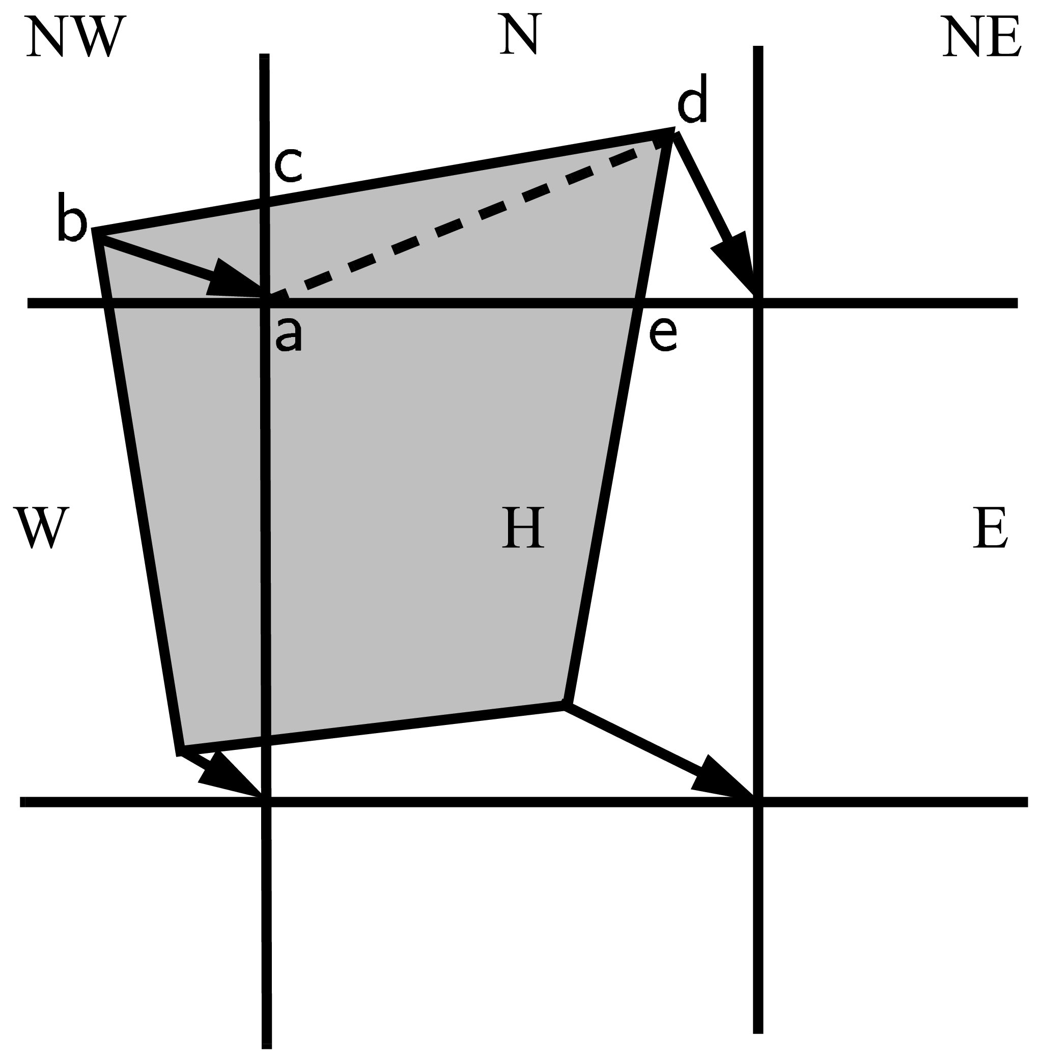
The method for locating departure triangles is discussed in detail by [7]. The basic idea is illustrated in Departure Region, which shows a shaded quadrilateral departure region whose contents are transported to the target or home grid cell, labeled \(H\). The neighboring grid cells are labeled by compass directions: \(NW\), \(N\), \(NE\), \(W\), and \(E\). The four vectors point along the velocity field at the cell corners, and the departure region is formed by joining the starting points of these vectors. Instead of integrating over the entire departure region, it is convenient to compute fluxes across cell edges. We identify departure regions for the north and east edges of each cell, which are also the south and west edges of neighboring cells. Consider the north edge of the home cell, across which there are fluxes from the neighboring \(NW\) and \(N\) cells. The contributing region from the \(NW\) cell is a triangle with vertices \(abc\), and that from the \(N\) cell is a quadrilateral that can be divided into two triangles with vertices \(acd\) and \(ade\). Focusing on triangle \(abc\), we first determine the coordinates of vertices \(b\) and \(c\) relative to the cell corner (vertex \(a\)), using Euclidean geometry to find vertex \(c\). Then we translate the three vertices to a coordinate system centered in the \(NW\) cell. This translation is needed in order to integrate fields (Section Integrating fields) in the coordinate system where they have been reconstructed (Section Reconstructing area and tracer fields). Repeating this process for the north and east edges of each grid cell, we compute the vertices of all the departure triangles associated with each cell edge.

Departure Region

Figure Departure Region shows that in incremental remapping, conserved quantities are remapped from the shaded departure region, a quadrilateral formed by connecting the backward trajectories from the four cell corners, to the grid cell labeled \(H\). The region fluxed across the north edge of cell \(H\) consists of a triangle (\(abc\)) in the \(NW\) cell and a quadrilateral (two triangles, \(acd\) and \(ade\)) in the \(N\) cell.

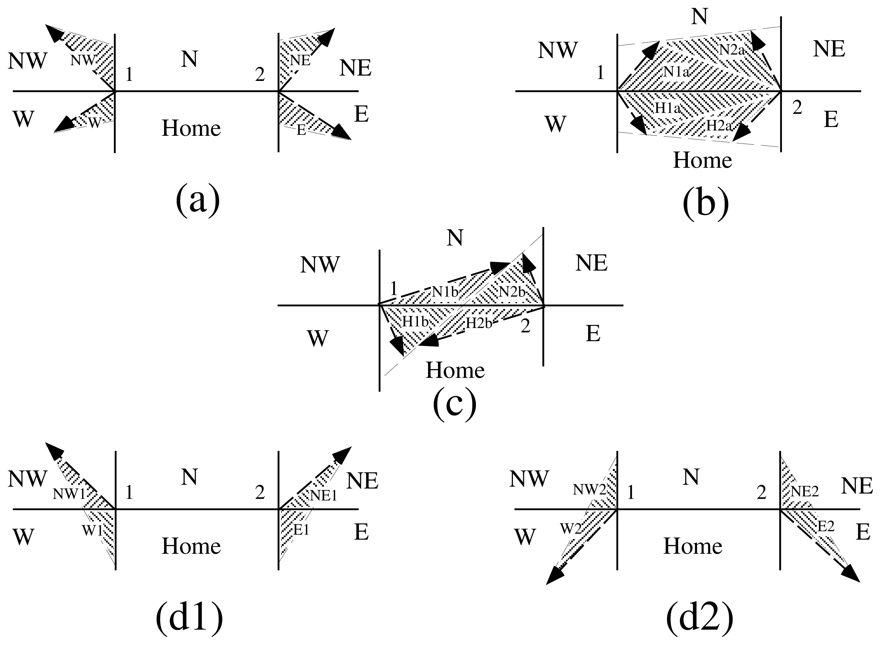
Figure Triangles, reproduced from [7], shows all possible triangles that can contribute fluxes across the north edge of a grid cell. There are 20 triangles, which can be organized into five groups of four mutually exclusive triangles as shown in Triangular Contributions. In this table, \((x_1, y_1)\) and \((x_2,y_2)\) are the Cartesian coordinates of the departure points relative to the northwest and northeast cell corners, respectively. The departure points are joined by a straight line that intersects the west edge at \((0,y_a)\) relative to the northwest corner and intersects the east edge at \((0,y_b)\) relative to the northeast corner. The east cell triangles and selecting conditions are identical except for a rotation through 90 degrees.

Triangles

Table Triangular Contributions show the evaluation of contributions from the 20 triangles across the north cell edge. The coordinates \(x_1\), \(x_2\), \(y_1\), \(y_2\), \(y_a\), and \(y_b\) are defined in the text. We define \(\tilde{y}_1 = y_1\) if \(x_1>0\), else \(\tilde{y}_1 = y_a\). Similarly, \(\tilde{y}_2 = y_2\) if \(x_2<0\), else \(\tilde{y}_2 = y_b\).

Triangular Contributions

Triangle group	Triangle label	Selecting logical condition
1	NW	\(y_a>0\) and \(y_1\geq0\) and \(x_1<0\)
	NW1	\(y_a<0\) and \(y_1\geq0\) and \(x_1<0\)
	W	\(y_a<0\) and \(y_1<0\) and \(x_1<0\)
	W2	\(y_a>0\) and \(y_1<0\) and \(x_1<0\)
2	NE	\(y_b>0\) and \(y_2\geq0\) and \(x_2>0\)
	NE1	\(y_b<0\) and \(y_2\geq0\) and \(x_2>0\)
	E	\(y_b<0\) and \(y_2<0\) and \(x_2>0\)
	E2	\(y_b>0\) and \(y_2<0\) and \(x_2>0\)
3	W1	\(y_a<0\) and \(y_1\geq0\) and \(x_1<0\)
	NW2	\(y_a>0\) and \(y_1<0\) and \(x_1<0\)
	E1	\(y_b<0\) and \(y_2\geq0\) and \(x_2>0\)
	NE2	\(y_b>0\) and \(y_2<0\) and \(x_2>0\)
4	H1a	\(y_a y_b\geq 0\) and \(y_a+y_b<0\)
	N1a	\(y_a y_b\geq 0\) and \(y_a+y_b>0\)
	H1b	\(y_a y_b<0\) and \(\tilde{y}_1<0\)
	N1b	\(y_a y_b<0\) and \(\tilde{y}_1>0\)
5	H2a	\(y_a y_b\geq 0\) and \(y_a+y_b<0\)
	N2a	\(y_a y_b\geq 0\) and \(y_a+y_b>0\)
	H2b	\(y_a y_b<0\) and \(\tilde{y}_2<0\)
	N2b	\(y_a y_b<0\) and \(\tilde{y}_2>0\)

This scheme was originally designed for rectangular grids. Grid cells in CICE actually lie on the surface of a sphere and must be projected onto a plane. The projection used in CICE maps each grid cell to a square with sides of unit length. Departure triangles across a given cell edge are computed in a coordinate system whose origin lies at the midpoint of the edge and whose vertices are at (-0.5, 0) and (0.5, 0). Intersection points are computed assuming Cartesian geometry with cell edges meeting at right angles. Let CL and CR denote the left and right vertices, which are joined by line CLR. Similarly, let DL and DR denote the departure points, which are joined by line DLR. Also, let IL and IR denote the intersection points (0, \(y_a\)) and (0, \(y_b\)) respectively, and let IC = (\(x_c\), 0) denote the intersection of CLR and DLR. It can be shown that \(y_a\), \(y_b\), and \(x_c\) are given by

\[\begin{split}\begin{aligned} y_a &=& {x_{CL} (y_{DM}-y_{DL}) + x_{DM}y_{DL} - x_{DL}y_{DM}}\over{x_{DM} - x_{DL}}, \\ y_b &=& {x_{CR} (y_{DR}-y_{DM}) - x_{DM}y_{DR} + x_{DR}y_{DM}}\over{x_{DR} - x_{DM}}, \\ x_c &=& x_{DL} - y_{DL} \left({x_{DR} - x_{DL}} \over y_{DR} - y_{DL}\right) \end{aligned}\end{split}\]

Each departure triangle is defined by three of the seven points (CL, CR, DL, DR, IL, IR, IC).

Given a 2D velocity field u, the divergence \(\nabla\cdot{\bf u}\) in a given grid cell can be computed from the local velocities and written in terms of fluxes across each cell edge:

(9)\[\nabla\cdot{\bf u} = {1\over A}\left[\left({u_{NE}+u_{SE}}\over 2\right)L_E + \left({u_{NW}+u_{SW}}\over 2\right)L_W + \left({u_{NE}+u_{NW}}\over 2\right)L_N + \left({u_{SE}+u_{SW}}\over 2\right)L_S \right],\]

where \(L\) is an edge length and the indices \(N, S, E, W\) denote compass directions. Equation (9) is equivalent to the divergence computed in the EVP dynamics (Section Dynamics). In general, the fluxes in this expression are not equal to those implied by the above scheme for locating departure regions. For some applications it may be desirable to prescribe the divergence by prescribing the area of the departure region for each edge. This can be done in CICE 4.0 by setting l_fixed_area = true in ice_transport_driver.F90 and passing the prescribed departure areas (edgearea_e and edgearea_n) into the remapping routine. An extra triangle is then constructed for each departure region to ensure that the total area is equal to the prescribed value. This idea was suggested and first implemented by Mats Bentsen of the Nansen Environmental and Remote Sensing Center (Norway), who applied an earlier version of the CICE remapping scheme to an ocean model. The implementation in CICE v4.0 is somewhat more general, allowing for departure regions lying on both sides of a cell edge. The extra triangle is constrained to lie in one but not both of the grid cells that share the edge. Since this option has yet to be fully tested in CICE, the current default is l_fixed_area = false.

We made one other change in the scheme of [7] for locating triangles. In their paper, departure points are defined by projecting cell corner velocities directly backward. That is,

(10)\[\mathbf{x_D} = -\mathbf{u} \, \Delta t,\]

where \(\mathbf{x}_D\) is the location of the departure point relative to the cell corner and \(\mathbf{u}\) is the velocity at the corner. This approximation is only first-order accurate. Accuracy can be improved by estimating the velocity at the midpoint of the trajectory.

2.4.3. Integrating fields

Next, we integrate the reconstructed fields over the departure triangles to find the total area, volume, and energy transported across each cell edge. Area transports are easy to compute since the area is linear in \(x\) and \(y\). Given a triangle with vertices \(\mathbf{x_i} = (x_i,y_i)\), \(i\in\{1,2,3\}\), the triangle area is

\[A_T = \frac{1}{2}\left|(x_2-x_1)(y_3-y_1) - (y_2-y_1)(x_3-x_1)\right|.\]

The integral \(F_a\) of any linear function \(f(\mathbf{r})\) over a triangle is given by

(11)\[F_a = A_T f(\mathbf{x_0}),\]

where \(\mathbf{x}_0 = (x_0,y_0)\) is the triangle midpoint,

\[\mathbf{x}_0={1\over 3}\sum_{i=1}^3\mathbf{x}_i.\]

To compute the area transport, we evaluate the area at the midpoint,

\[a(\mathbf{x}_0) = a_c + a_x x_0 + a_y y_0,\]

and multiply by \(A_T\). By convention, northward and eastward transport is positive, while southward and westward transport is negative.

Equation (11) cannot be used for volume transport, because the reconstructed volumes are quadratic functions of position. (They are products of two linear functions, area and thickness.) The integral of a quadratic polynomial over a triangle requires function evaluations at three points,

(12)\[F_h = \frac{A_T}{3}\sum_{i=1}^3 f\left({\mathbf x}^\prime_i\right),\]

where \(\mathbf{x}_i^\prime = (\mathbf{x}_0+\mathbf{x}_i)/2\) are points lying halfway between the midpoint and the three vertices. [7] use this formula to compute transports of the product \(\rho \, T\), which is analogous to ice volume. Equation (12) does not work for ice and snow energies, which are cubic functions—products of area, thickness, and enthalpy. Integrals of a cubic polynomial over a triangle can be evaluated using a four-point formula [45]:

(13)\[F_q = A_T \left[ -\frac{9}{16} f(\mathbf{x}_0) + \frac{25}{48} \sum_{i=1}^3 f(\mathbf{x}_i^{\prime\prime})\right]\]

where \(\mathbf{x_i}^{\prime\prime}=(3 \mathbf{x}_0 + 2 \mathbf{x}_i)/5\). To evaluate functions at specific points, we must compute many products of the form \(a({\bf x}) \, h({\bf x})\) and \(a({\bf x}) \, h({\bf x}) \, q({\bf x})\), where each term in the product is the sum of a cell-center value and two displacement terms. In the code, the computation is sped up by storing some sums that are used repeatedly.

2.4.4. Updating state variables

Finally, we compute new values of the state variables in each ice category and grid cell. The new fractional ice areas \(a_{in}^\prime(i,j)\) are given by

(14)\[a_{in}^\prime(i,j) = a_{in}(i,j) + \frac{F_{aE}(i-1,j) - F_{aE}(i,j) + F_{aN}(i,j-1) - F_{aN}(i,j)} {A(i,j)}\]

where \(F_{aE}(i,j)\) and \(F_{aN}(i,j)\) are the area transports across the east and north edges, respectively, of cell \((i,j)\), and \(A(i,j)\) is the grid cell area. All transports added to one cell are subtracted from a neighboring cell; thus Equation (14) conserves total ice area.

The new ice volumes and energies are computed analogously. New thicknesses are given by the ratio of volume to area, and enthalpies by the ratio of energy to volume. Tracer monotonicity is ensured because

\[h^\prime = {\int_A a \, h \, dA \over \int_A a \, dA},\]

\[q^\prime = {\int_A a \, h \, q\,dA \over \int_A a \, h \ dA},\]

where \(h^\prime\) and \(q^\prime\) are the new-time thickness and enthalpy, given by integrating the old-time ice area, volume, and energy over a Lagrangian departure region with area \(A\). That is, the new-time thickness and enthalpy are weighted averages over old-time values, with non-negative weights \(a\) and \(ah\). Thus the new-time values must lie between the maximum and minimum of the old-time values.