3.1. Implementation
CICE is written in FORTRAN90 and runs on platforms using UNIX, LINUX, and other operating systems. The code is based on a two-dimensional horizontal orthogonal grid that is broken into two-dimensional horizontal blocks and parallelized over blocks with MPI and OpenMP threads. The code also includes some optimizations for vector architectures.
CICE consists of source code under the cicecore/ directory that supports model dynamics and top-level control. The column physics source code is under the icepack/ directory and this is implemented as a submodule in github from a separate repository (CICE) There is also a configuration/ directory that includes scripts for configuring CICE cases.
3.1.1. Directory structure
The present code distribution includes source code and scripts. Forcing data is available from the ftp site. The directory structure of CICE is as follows
- LICENSE.pdf
license for using and sharing the code
- DistributionPolicy.pdf
policy for using and sharing the code
- README.md
basic information and pointers
- icepack/
the Icepack module. The icepack subdirectory includes Icepack specific scripts, drivers, and documentation. CICE only uses the columnphysics source code under icepack/columnphysics/.
- cicecore/
CICE source code
- cicecore/cicedynB/
routines associated with the dynamics core
- cicecore/drivers/
top-level CICE drivers and coupling layers
- cicecore/shared/
CICE source code that is independent of the dynamical core
- cicecore/version.txt
file that indicates the CICE model version.
- configuration/scripts/
support scripts, see Scripts
- doc/
documentation
- cice.setup
main CICE script for creating cases
- dot files
various files that begin with . and store information about the git repository or other tools.
A case (compile) directory is created upon initial execution of the script
cice.setup at the user-specified location provided after the -c flag.
Executing the command ./cice.setup -h provides helpful information for
this tool.
3.1.2. Grid, boundary conditions and masks
The spatial discretization is specialized for a generalized orthogonal B-grid as in [34] or [44]. The ice and snow area, volume and energy are given at the center of the cell, velocity is defined at the corners, and the internal ice stress tensor takes four different values within a grid cell; bilinear approximations are used for the stress tensor and the ice velocity across the cell, as described in [18]. This tends to avoid the grid decoupling problems associated with the B-grid. EVP is available on the C-grid through the MITgcm code distribution, http://mitgcm.org/viewvc/MITgcm/MITgcm/pkg/seaice/.
Since ice thickness and thermodynamic variables such as temperature are given in the center of each cell, the grid cells are referred to as “T cells.” We also occasionally refer to “U cells,” which are centered on the northeast corner of the corresponding T cells and have velocity in the center of each. The velocity components are aligned along grid lines.
The user has several choices of grid routines: popgrid reads grid lengths and other parameters for a nonuniform grid (including tripole and regional grids), and rectgrid creates a regular rectangular grid. The input files global_gx3.grid and global_gx3.kmt contain the \(\left<3^\circ\right>\) POP grid and land mask; global_gx1.grid and global_gx1.kmt contain the \(\left<1^\circ\right>\) grid and land mask, and global_tx1.grid and global_tx1.kmt contain the \(\left<1^\circ\right>\) POP tripole grid and land mask. These are binary unformatted, direct access, Big Endian files.
In CESM, the sea ice model may exchange coupling fluxes using a
different grid than the computational grid. This functionality is
activated using the namelist variable gridcpl_file.
3.1.2.1. Grid domains and blocks
In general, the global gridded domain is
nx_global \(\times\)ny_global, while the subdomains used in the
block distribution are nx_block \(\times\)ny_block. The
physical portion of a subdomain is indexed as [ilo:ihi, jlo:jhi], with
nghost “ghost” or “halo” cells outside the domain used for boundary
conditions. These parameters are illustrated in Grid parameters in one
dimension. The routines global_scatter and global_gather
distribute information from the global domain to the local domains and
back, respectively. If MPI is not being used for grid decomposition in
the ice model, these routines simply adjust the indexing on the global
domain to the single, local domain index coordinates. Although we
recommend that the user choose the local domains so that the global
domain is evenly divided, if this is not possible then the furthest east
and/or north blocks will contain nonphysical points (“padding”). These
points are excluded from the computation domain and have little effect
on model performance.
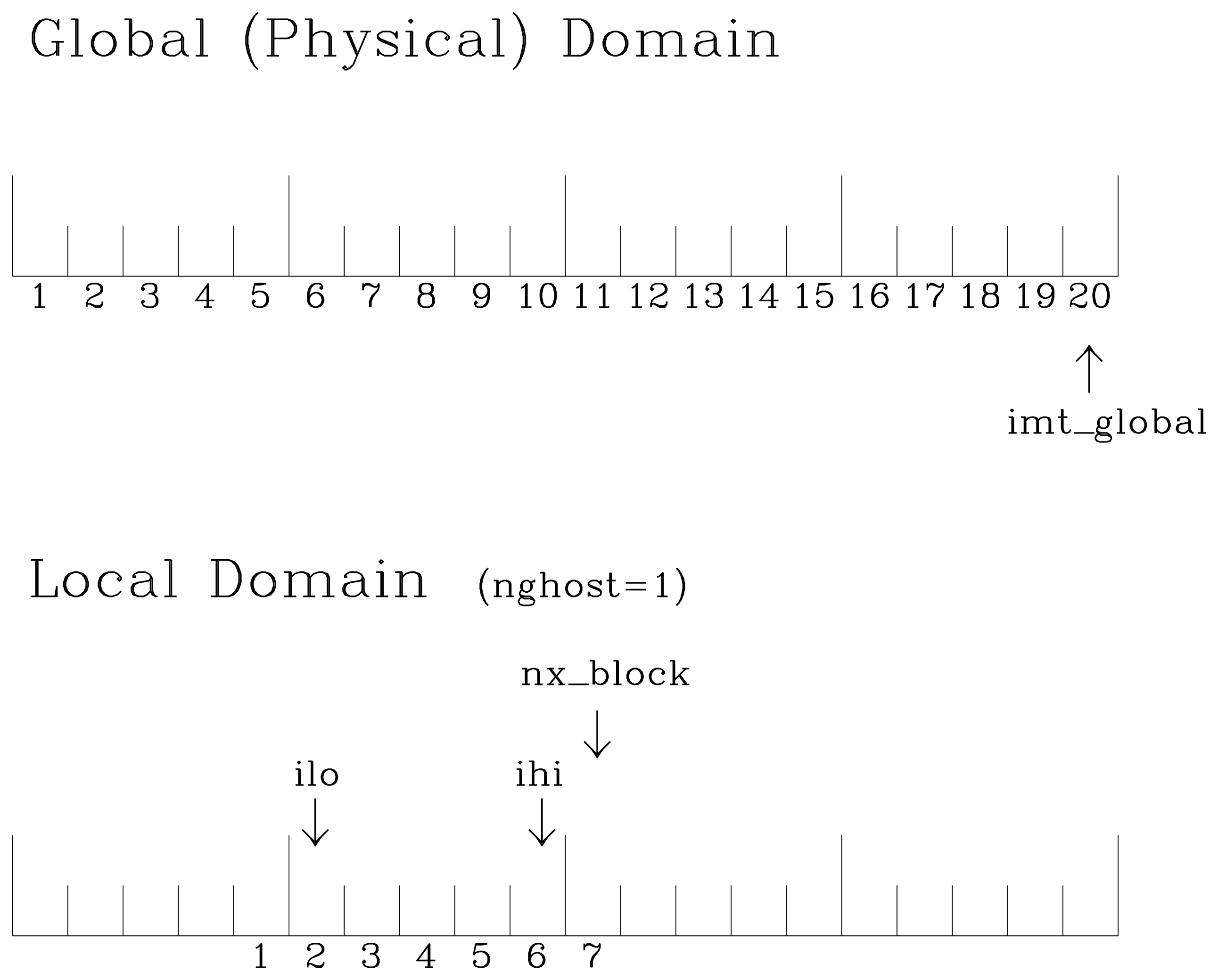
Grid parameters
Figure Grid parameters shows the grid parameters for a sample one-dimensional, 20-cell
global domain decomposed into four local subdomains. Each local
domain has one ghost (halo) cell on each side, and the physical
portion of the local domains are labeled ilo:ihi. The parameter
nx_block is the total number of cells in the local domain, including
ghost cells, and the same numbering system is applied to each of the
four subdomains.
The user sets the NTASKS and NTHRDS settings in cice.settings
and chooses a block size block_size_x \(\times\)block_size_y,
max_blocks, and decomposition information distribution_type, processor_shape,
and distribution_type in ice_in. That information is used to
determine how the blocks are
distributed across the processors, and how the processors are
distributed across the grid domain. Recommended combinations of these
parameters for best performance are given in Section Performance.
The script cice.setup computes some default decompositions and layouts
but the user can overwrite the defaults by manually changing the values in
ice_in. At runtime, the model will print decomposition
information to the log file, and if the block size or max blocks is
inconsistent with the task and thread size, the model will abort. The
code will also print a warning if the maximum number of blocks is too large.
Although this is not fatal, it does use extra memory. If max_blocks is
set to -1, the code will compute a max_blocks on the fly.
A loop at the end of routine create_blocks in module
ice_blocks.F90 will print the locations for all of the blocks on
the global grid if dbug is set to be true. Likewise, a similar loop at
the end of routine create_local_block_ids in module
ice_distribution.F90 will print the processor and local block
number for each block. With this information, the grid decomposition
into processors and blocks can be ascertained. The dbug flag must be
manually set in the code in each case (independently of the dbug flag in
ice_in), as there may be hundreds or thousands of blocks to print
and this information should be needed only rarely. This information is
much easier to look at using a debugger such as Totalview. There is also
an output field that can be activated in icefields_nml, f_blkmask,
that prints out the variable blkmask to the history file and
which labels the blocks in the grid decomposition according to blkmask =
my_task + iblk/100.
3.1.2.2. Tripole grids
The tripole grid is a device for constructing a global grid with a
normal south pole and southern boundary condition, which avoids placing
a physical boundary or grid singularity in the Arctic Ocean. Instead of
a single north pole, it has two “poles” in the north, both located on
land, with a line of grid points between them. This line of points is
called the “fold,” and it is the “top row” of the physical grid. One
pole is at the left-hand end of the top row, and the other is in the
middle of the row. The grid is constructed by “folding” the top row, so
that the left-hand half and the right-hand half of it coincide. Two
choices for constructing the tripole grid are available. The one first
introduced to CICE is called “U-fold”, which means that the poles and
the grid cells between them are U cells on the grid. Alternatively the
poles and the cells between them can be grid T cells, making a “T-fold.”
Both of these options are also supported by the OPA/NEMO ocean model,
which calls the U-fold an “f-fold” (because it uses the Arakawa C-grid
in which U cells are on T-rows). The choice of tripole grid is given by
the namelist variable ns_boundary_type, ‘tripole’ for the U-fold and
‘tripoleT’ for the T-fold grid.
In the U-fold tripole grid, the poles have U-index
\({\tt nx\_global}/2\) and nx_global on the top U-row of the
physical grid, and points with U-index i and \({\tt nx\_global-i}\)
are coincident. Let the fold have U-row index \(n\) on the global
grid; this will also be the T-row index of the T-row to the south of the
fold. There are ghost (halo) T- and U-rows to the north, beyond the
fold, on the logical grid. The point with index i along the ghost T-row
of index \(n+1\) physically coincides with point
\({\tt nx\_global}-{\tt i}+1\) on the T-row of index \(n\). The
ghost U-row of index \(n+1\) physically coincides with the U-row of
index \(n-1\).
In the T-fold tripole grid, the poles have T-index 1 and and \({\tt nx\_global}/2+1\) on the top T-row of the physical grid, and points with T-index i and \({\tt nx\_global}-{\tt i}+2\) are coincident. Let the fold have T-row index \(n\) on the global grid. It is usual for the northernmost row of the physical domain to be a U-row, but in the case of the T-fold, the U-row of index \(n\) is “beyond” the fold; although it is not a ghost row, it is not physically independent, because it coincides with U-row \(n-1\), and it therefore has to be treated like a ghost row. Points i on U-row \(n\) coincides with \({\tt nx\_global}-{\tt i}+1\) on U-row \(n-1\). There are still ghost T- and U-rows \(n+1\) to the north of U-row \(n\). Ghost T-row \(n+1\) coincides with T-row \(n-1\), and ghost U-row \(n+1\) coincides with U-row \(n-2\).
The tripole grid thus requires two special kinds of treatment for certain rows, arranged by the halo-update routines. First, within rows along the fold, coincident points must always have the same value. This is achieved by averaging them in pairs. Second, values for ghost rows and the “quasi-ghost” U-row on the T-fold grid are reflected copies of the coincident physical rows. Both operations involve the tripole buffer, which is used to assemble the data for the affected rows. Special treatment is also required in the scattering routine, and when computing global sums one of each pair of coincident points has to be excluded.
3.1.2.3. Vertical Grids
The sea ice physics described in a single column or grid cell is contained in the Icepack submodule, which can be run independently of the CICE model. Icepack includes a vertical grid for the physics and a “bio-grid” for biogeochemistry, described in the Icepack Documentation. History variables available for column output are ice and snow temperature, Tinz and Tsnz, and the ice salinity profile, Sinz. These variables also include thickness category as a fourth dimension.
3.1.2.4. Boundary conditions
Much of the infrastructure used in CICE, including the boundary routines, is adopted from POP. The boundary routines perform boundary communications among processors when MPI is in use and among blocks whenever there is more than one block per processor.
Open/cyclic boundary conditions are the default in CICE; the physical
domain can still be closed using the land mask. In our bipolar,
displaced-pole grids, one row of grid cells along the north and south
boundaries is located on land, and along east/west domain boundaries not
masked by land, periodic conditions wrap the domain around the globe.
CICE can be run on regional grids with open boundary conditions; except
for variables describing grid lengths, non-land halo cells along the
grid edge must be filled by restoring them to specified values. The
namelist variable restore_ice turns this functionality on and off; the
restoring timescale trestore may be used (it is also used for restoring
ocean sea surface temperature in stand-alone ice runs). This
implementation is only intended to provide the “hooks” for a more
sophisticated treatment; the rectangular grid option can be used to test
this configuration. The ‘displaced_pole’ grid option should not be used
unless the regional grid contains land all along the north and south
boundaries. The current form of the boundary condition routines does not
allow Neumann boundary conditions, which must be set explicitly. This
has been done in an unreleased branch of the code; contact Elizabeth for
more information.
For exact restarts using restoring, set restart_ext = true in namelist
to use the extended-grid subroutines.
On tripole grids, the order of operations used for calculating elements of the stress tensor can differ on either side of the fold, leading to round-off differences. Although restarts using the extended grid routines are exact for a given run, the solution will differ from another run in which restarts are written at different times. For this reason, explicit halo updates of the stress tensor are implemented for the tripole grid, both within the dynamics calculation and for restarts. This has not been implemented yet for tripoleT grids, pending further testing.
3.1.2.5. Masks
A land mask hm (\(M_h\)) is specified in the cell centers, with 0 representing land and 1 representing ocean cells. A corresponding mask uvm (\(M_u\)) for velocity and other corner quantities is given by
The logical masks tmask and umask (which correspond to the real masks
hm and uvm, respectively) are useful in conditional statements.
In addition to the land masks, two other masks are implemented in
dyn_prep in order to reduce the dynamics component’s work on a global
grid. At each time step the logical masks ice_tmask and ice_umask are
determined from the current ice extent, such that they have the value
“true” wherever ice exists. They also include a border of cells around
the ice pack for numerical purposes. These masks are used in the
dynamics component to prevent unnecessary calculations on grid points
where there is no ice. They are not used in the thermodynamics
component, so that ice may form in previously ice-free cells. Like the
land masks hm and uvm, the ice extent masks ice_tmask and ice_umask
are for T cells and U cells, respectively.
Improved parallel performance may result from utilizing halo masks for
boundary updates of the full ice state, incremental remapping transport,
or for EVP or EAP dynamics. These options are accessed through the
logical namelist flags maskhalo_bound, maskhalo_remap, and
maskhalo_dyn, respectively. Only the halo cells containing needed
information are communicated.
Two additional masks are created for the user’s convenience: lmask_n
and lmask_s can be used to compute or write data only for the northern
or southern hemispheres, respectively. Special constants (spval and
spval_dbl, each equal to \(10^{30}\)) are used to indicate land
points in the history files and diagnostics.
3.1.2.6. Performance
Namelist options (domain_nml) provide considerable flexibility for
finding efficient processor and block configuration. Some of
these choices are illustrated in Distribution options. Users have control
of many aspects of the decomposition such as the block size (block_size_x,
block_size_y), the distribution_type, the distribution_wght,
the distribution_wght_file (when distribution_type = wghtfile),
and the processor_shape (when distribution_type = cartesian).
The user specifies the total number of tasks and threads in cice.settings and the block size and decompostion in the namelist file. The main trades offs are the relative efficiency of large square blocks versus model internal load balance as CICE computation cost is very small for ice-free blocks. Smaller, more numerous blocks provides an opportunity for better load balance by allocating each processor both ice-covered and ice-free blocks. But smaller, more numerous blocks becomes less efficient due to MPI communication associated with halo updates. In practice, blocks should probably not have fewer than about 8 to 10 grid cells in each direction, and more square blocks tend to optimize the volume-to-surface ratio important for communication cost. Often 3 to 8 blocks per processor provide the decompositions flexiblity to create reasonable load balance configurations.
The distribution_type options allow standard cartesian distributions
of blocks, redistribution via a ‘rake’ algorithm for improved load
balancing across processors, and redistribution based on space-filling
curves. There are also additional distribution types
(‘roundrobin,’ ‘sectrobin,’ ‘sectcart’, and ‘spiralcenter’) that support
alternative decompositions and also allow more flexibility in the number of
processors used. Finally, there is a ‘wghtfile’ decomposition that
generates a decomposition based on weights specified in an input file.
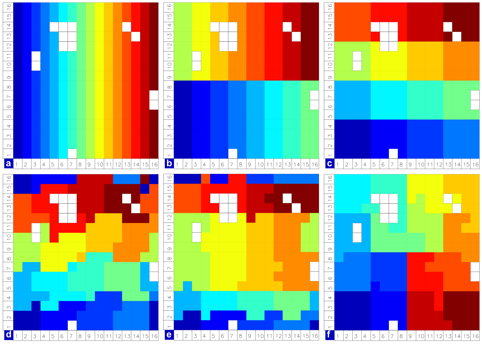
Distribution options
Figure Distribution options shows distribution of 256 blocks across 16 processors, represented by colors, on the gx1 grid: (a) cartesian, slenderX1, (b) cartesian, slenderX2, (c) cartesian, square-ice (square-pop is equivalent here), (d) rake with block weighting, (e) rake with latitude weighting, (f) spacecurve. Each block consists of 20x24 grid cells, and white blocks consist entirely of land cells.
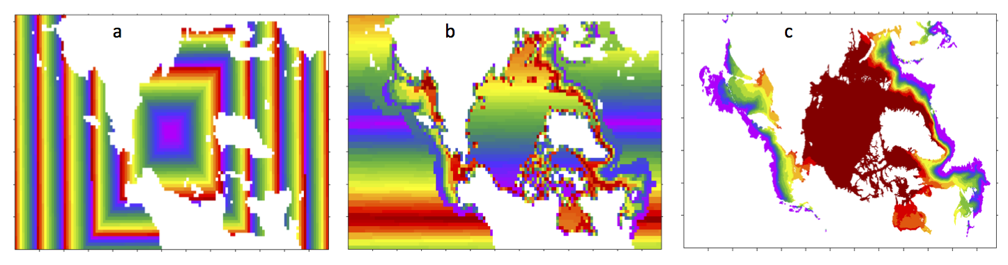
Decomposition options
Figure Decomposition options shows sample decompositions for (a) spiral center and (b) wghtfile for an Arctic polar grid. (c) is the weight field in the input file use to drive the decompostion in (b).
processor_shape is used with the distribution_type cartesian option,
and it allocates blocks to processors in various groupings such as
tall, thin processor domains (slenderX1 or slenderX2,
often better for sea ice simulations on global grids where nearly all of
the work is at the top and bottom of the grid with little to do in
between) and close-to-square domains (square-pop or square-ice),
which maximize the volume to
surface ratio (and therefore on-processor computations to message
passing, if there were ice in every grid cell). In cases where the
number of processors is not a perfect square (4, 9, 16…), the
processor_shape namelist variable allows the user to choose how the
processors are arranged. Here again, it is better in the sea ice model
to have more processors in x than in y, for example, 8 processors
arranged 4x2 (square-ice) rather than 2x4 (square-pop). The latter
option is offered for direct-communication compatibility with POP, in
which this is the default.
distribution_wght chooses how the work-per-block estimates are
weighted. The ‘block’ option is the default in POP and it weights each
block equally. This is useful in POP which always has work in
each block and is written with a lot of
array syntax requiring calculations over entire blocks (whether or not
land is present). This option is provided in CICE as well for
direct-communication compatibility with POP. The ‘latitude’ option
weights the blocks based on latitude and the number of ocean grid
cells they contain. Many of the non-cartesian decompositions support
automatic land block elimination and provide alternative ways to
decompose blocks without needing the distribution_wght.
The rake distribution type is initialized as a standard, Cartesian distribution. Using the work-per-block estimates, blocks are “raked” onto neighboring processors as needed to improve load balancing characteristics among processors, first in the x direction and then in y.
Space-filling curves reduce a multi-dimensional space (2D, in our case) to one dimension. The curve is composed of a string of blocks that is snipped into sections, again based on the work per processor, and each piece is placed on a processor for optimal load balancing. This option requires that the block size be chosen such that the number of blocks in the x direction and the number of blocks in the y direction must be factorable as \(2^n 3^m 5^p\) where \(n, m, p\) are integers. For example, a 16x16 array of blocks, each containing 20x24 grid cells, fills the gx1 grid (\(n=4, m=p=0\)). If either of these conditions is not met, the spacecurve decomposition will fail.
While the Cartesian distribution groups sets of blocks by processor, the ‘roundrobin’ distribution loops through the blocks and processors together, putting one block on each processor until the blocks are gone. This provides good load balancing but poor communication characteristics due to the number of neighbors and the amount of data needed to communicate. The ‘sectrobin’ and ‘sectcart’ algorithms loop similarly, but put groups of blocks on each processor to improve the communication characteristics. In the ‘sectcart’ case, the domain is divided into four (east-west,north-south) quarters and the loops are done over each, sequentially.
The wghtfile decomposition drives the decomposition based on
weights provided in a weight file. That file should be a netcdf
file with a double real field called wght containing the relative
weight of each gridcell. Decomposition options (b) and (c) show
an example. The weights associated with each gridcell will be
summed on a per block basis and normalized to about 10 bins to
carry out the distribution of highest to lowest block weights
to processors. Scorecard provides an overview
of the pros and cons of the various distribution types.

Scorecard
Figure Scorecard shows the scorecard for block distribution choices in CICE, courtesy T. Craig. For more information, see [6] or http://www.cesm.ucar.edu/events/workshops/ws.2012/presentations/sewg/craig.pdf
The maskhalo options in the namelist improve performance by removing
unnecessary halo communications where there is no ice. There is some
overhead in setting up the halo masks, which is done during the
timestepping procedure as the ice area changes, but this option
usually improves timings even for relatively small processor counts.
T. Craig has found that performance improved by more than 20% for
combinations of updated decompositions and masked haloes, in CESM’s
version of CICE.
Throughout the code, (i, j) loops have been combined into a single loop, often over just ocean cells or those containing sea ice. This was done to reduce unnecessary operations and to improve vector performance.
Timings illustrates the CICE v5 computational expense of various options, relative to the total time (excluding initialization) of a 7-layer configuration using BL99 thermodynamics, EVP dynamics, and the ‘ccsm3’ shortwave parameterization on the gx1 grid, run for one year from a no-ice initial condition. The block distribution consisted of 20 \(\times\) 192 blocks spread over 32 processors (‘slenderX2’) with no threads and -O2 optimization. Timings varied by about \(\pm3\)% in identically configured runs due to machine load. Extra time required for tracers has two components, that needed to carry the tracer itself (advection, category conversions) and that needed for the calculations associated with the particular tracer. The age tracers (FY and iage) require very little extra calculation, so their timings represent essentially the time needed just to carry an extra tracer. The topo melt pond scheme is slightly faster than the others because it calculates pond area and volume once per grid cell, while the others calculate it for each thickness category.
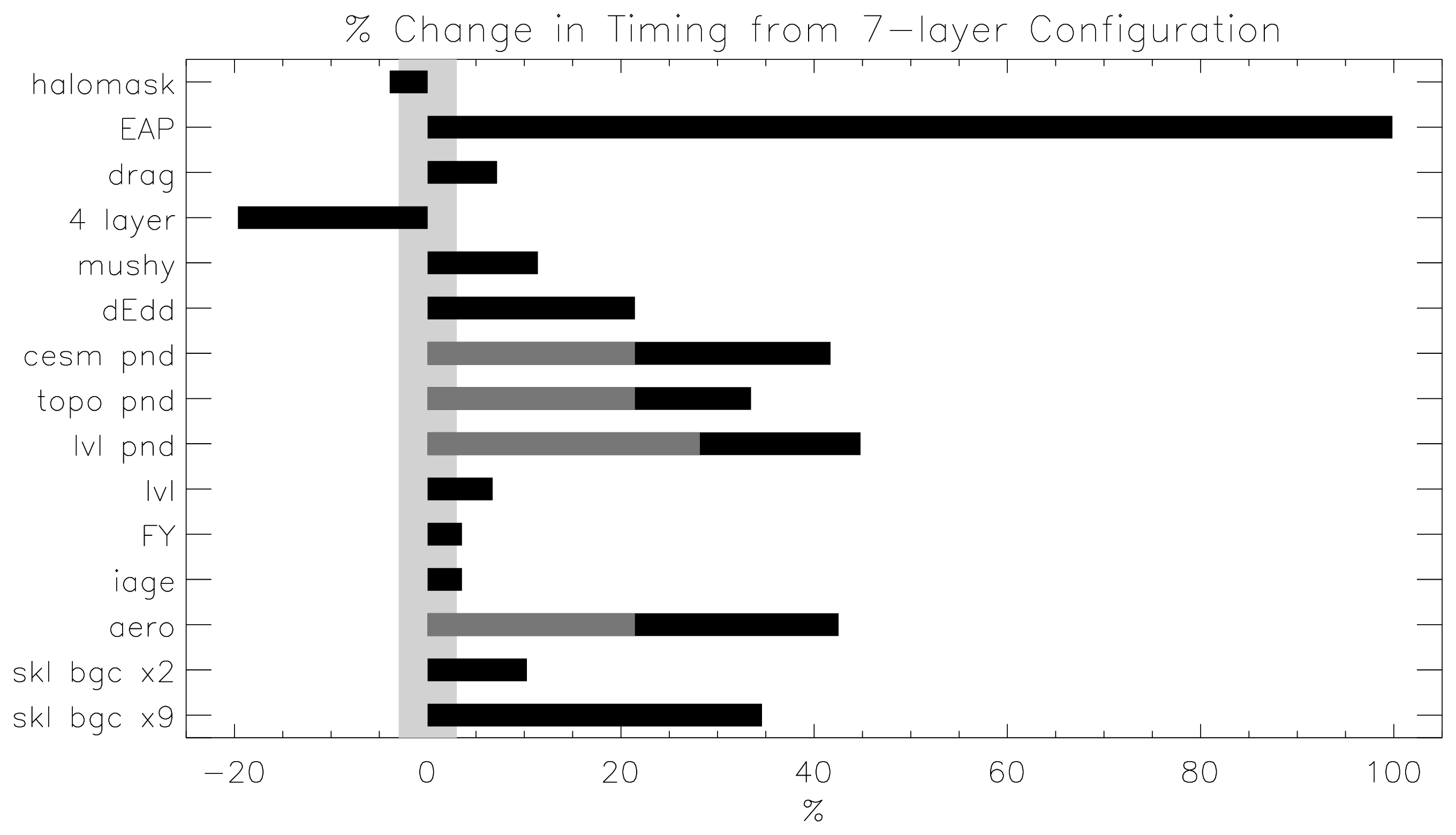
Timings
Figure Timings shows change in ‘TimeLoop’ timings from the 7-layer configuration using BL99 thermodynamics and EVP dynamics. Timings were made on a nondedicated machine, with variations of about \(\pm3\)% in identically configured runs (light grey). Darker grey indicates the time needed for extra required options; The Delta-Eddington radiation scheme is required for all melt pond schemes and the aerosol tracers, and the level-ice pond parameterization additionally requires the level-ice tracers.
3.1.3. Initialization and coupling
The ice model’s parameters and variables are initialized in several steps. Many constants and physical parameters are set in ice_constants.F90. Namelist variables (Table of namelist options), whose values can be altered at run time, are handled in input_data and other initialization routines. These variables are given default values in the code, which may then be changed when the input file ice_in is read. Other physical constants, numerical parameters, and variables are first set in initialization routines for each ice model component or module. Then, if the ice model is being restarted from a previous run, core variables are read and reinitialized in restartfile, while tracer variables needed for specific configurations are read in separate restart routines associated with each tracer or specialized parameterization. Finally, albedo and other quantities dependent on the initial ice state are set. Some of these parameters will be described in more detail in Table of namelist options.
The restart files supplied with the code release include the core
variables on the default configuration, that is, with seven vertical
layers and the ice thickness distribution defined by kcatbound = 0.
Restart information for some tracers is also included in the netCDF restart
files.
Three namelist variables control model initialization, ice_ic, runtype,
and restart, as described in Ice Initial State. It is possible to do an
initial run from a file filename in two ways: (1) set runtype =
‘initial’, restart = true and ice_ic = filename, or (2) runtype =
‘continue’ and pointer_file = ./restart/ice.restart_file where
./restart/ice.restart_file contains the line
“./restart/[filename]”. The first option is convenient when repeatedly
starting from a given file when subsequent restart files have been
written. With this arrangement, the tracer restart flags can be set to
true or false, depending on whether the tracer restart data exist. With
the second option, tracer restart flags are set to ‘continue’ for all
active tracers.
An additional namelist option, restart_ext specifies whether halo cells
are included in the restart files. This option is useful for tripole and
regional grids, but can not be used with PIO.
MPI is initialized in init_communicate for both coupled and stand-alone MPI runs. The ice component communicates with a flux coupler or other climate components via external routines that handle the variables listed in the Icepack documentation. For stand-alone runs, routines in ice_forcing.F90 read and interpolate data from files, and are intended merely to provide guidance for the user to write his or her own routines. Whether the code is to be run in stand-alone or coupled mode is determined at compile time, as described below.
Table Ice Initial State shows ice initial state resulting from combinations of
ice_ic, runtype and restart. \(^a\)If false, restart is reset to
true. \(^b\)restart is reset to false. \(^c\)ice_ic is
reset to ‘none.’
ice_ic |
|||
|---|---|---|---|
initial/false |
initial/true |
continue/true (or false\(^a\)) |
|
none |
no ice |
no ice\(^b\) |
restart using pointer_file |
default |
SST/latitude dependent |
SST/latitude dependent\(^b\) |
restart using pointer_file |
filename |
no ice\(^c\) |
start from filename |
restart using pointer_file |
3.1.4. Choosing an appropriate time step
The time step is chosen based on stability of the transport component
(both horizontal and in thickness space) and on resolution of the
physical forcing. CICE allows the dynamics, advection and ridging
portion of the code to be run with a shorter timestep,
\(\Delta t_{dyn}\) (dt_dyn), than the thermodynamics timestep
\(\Delta t\) (dt). In this case, dt and the integer ndtd are
specified, and dt_dyn = dt/ndtd.
A conservative estimate of the horizontal transport time step bound, or CFL condition, under remapping yields
Numerical estimates for this bound for several POP grids, assuming \(\max(u, v)=0.5\) m/s, are as follows:
grid label |
N pole singularity |
dimensions |
min \(\sqrt{\Delta x\cdot\Delta y}\) |
max \(\Delta t_{dyn}\) |
gx3 |
Greenland |
\(100\times 116\) |
\(39\times 10^3\) m |
10.8hr |
gx1 |
Greenland |
\(320\times 384\) |
\(18\times 10^3\) m |
5.0hr |
p4 |
Canada |
\(900\times 600\) |
\(6.5\times 10^3\) m |
1.8hr |
As discussed in [31], the maximum time step in practice is
usually determined by the time scale for large changes in the ice
strength (which depends in part on wind strength). Using the strength
parameterization of [42], limits the time step to \(\sim\)30
minutes for the old ridging scheme (krdg_partic = 0), and to
\(\sim\)2 hours for the new scheme (krdg_partic = 1), assuming
\(\Delta x\) = 10 km. Practical limits may be somewhat less,
depending on the strength of the atmospheric winds.
Transport in thickness space imposes a similar restraint on the time step, given by the ice growth/melt rate and the smallest range of thickness among the categories, \(\Delta t<\min(\Delta H)/2\max(f)\), where \(\Delta H\) is the distance between category boundaries and \(f\) is the thermodynamic growth rate. For the 5-category ice thickness distribution used as the default in this distribution, this is not a stringent limitation: \(\Delta t < 19.4\) hr, assuming \(\max(f) = 40\) cm/day.
In the classic EVP or EAP approach (kdyn = 1 or 2, revised_evp = false),
the dynamics component is subcycled ndte (\(N\)) times per dynamics
time step so that the elastic waves essentially disappear before the
next time step. The subcycling time step (\(\Delta
t_e\)) is thus
A second parameter, \(E_\circ\) (eyc), defines the elastic wave
damping timescale \(T\), described in Section Dynamics, as
eyc * dt_dyn. The forcing terms are not updated during the subcycling.
Given the small step (dte) at which the EVP dynamics model is subcycled,
the elastic parameter \(E\) is also limited by stability
constraints, as discussed in [17]. Linear stability
analysis for the dynamics component shows that the numerical method is
stable as long as the subcycling time step \(\Delta t_e\)
sufficiently resolves the damping timescale \(T\). For the stability
analysis we had to make several simplifications of the problem; hence
the location of the boundary between stable and unstable regions is
merely an estimate. In practice, the ratio
\(\Delta t_e ~:~ T ~:~ \Delta t\) = 1 : 40 : 120 provides both
stability and acceptable efficiency for time steps (\(\Delta t\)) on
the order of 1 hour.
Note that only \(T\) and \(\Delta t_e\) figure into the stability of the dynamics component; \(\Delta t\) does not. Although the time step may not be tightly limited by stability considerations, large time steps (e.g., \(\Delta t=1\) day, given daily forcing) do not produce accurate results in the dynamics component. The reasons for this error are discussed in [17]; see [21] for its practical effects. The thermodynamics component is stable for any time step, as long as the surface temperature \(T_{sfc}\) is computed internally. The numerical constraint on the thermodynamics time step is associated with the transport scheme rather than the thermodynamic solver.
For the revised EVP approach (kdyn = 1, revised_evp = true), the
relaxation parameter arlx1i effectively sets the damping timescale in
the problem, and brlx represents the effective subcycling
[4] (see Section Revised approach).
3.1.5. Model output
3.1.5.1. History files
Model output data is averaged over the period(s) given by histfreq and
histfreq_n, and written to binary or netCDF files prepended by history_file
in ice_in. These settings for history files are set in the
setup_nml section of ice_in (see Table of namelist options).
If history_file = ‘iceh’ then the
filenames will have the form iceh.[timeID].nc or iceh.[timeID].da,
depending on the output file format chosen in cice.settings (set
ICE_IOTYPE). The netCDF history files are CF-compliant; header information for
data contained in the netCDF files is displayed with the command ncdump -h
filename.nc. Parallel netCDF output is available using the PIO library; the
attribute io_flavor distinguishes output files written with PIO from
those written with standard netCDF. With binary files, a separate header
file is written with equivalent information. Standard fields are output
according to settings in the icefields_nml section of ice_in
(see Table of namelist options).
The user may add (or subtract) variables not already available in the
namelist by following the instructions in section Adding History fields.
The history module has been divided into several modules based on the desired formatting and on the variables themselves. Parameters, variables and routines needed by multiple modules is in ice_history_shared.F90, while the primary routines for initializing and accumulating all of the history variables are in ice_history.F90. These routines call format-specific code in the io_binary, io_netcdf and io_pio directories. History variables specific to certain components or parameterizations are collected in their own history modules (ice_history_bgc.F90, ice_history_drag.F90, ice_history_mechred.F90, ice_history_pond.F90).
The history modules allow output at different frequencies. Five output
frequencies (1, h, d, m, y) are available simultaneously during a run.
The same variable can be output at different frequencies (say daily and
monthly) via its namelist flag, f_ \(\left<{var}\right>\), which
is now a character string corresponding to histfreq or ‘x’ for none.
(Grid variable flags are still logicals, since they are written to all
files, no matter what the frequency is.) If there are no namelist flags
with a given histfreq value, or if an element of histfreq_n is 0, then
no file will be written at that frequency. The output period can be
discerned from the filenames.
For example, in the namelist:
``histfreq`` = ’1’, ’h’, ’d’, ’m’, ’y’
``histfreq_n`` = 1, 6, 0, 1, 1
``f_hi`` = ’1’
``f_hs`` = ’h’
``f_Tsfc`` = ’d’
``f_aice`` = ’m’
``f_meltb`` = ’mh’
``f_iage`` = ’x’
Here, hi will be written to a file on every timestep, hs will be
written once every 6 hours, aice once a month, meltb once a month AND
once every 6 hours, and Tsfc and iage will not be written.
From an efficiency standpoint, it is best to set unused frequencies in
histfreq to ‘x’. Having output at all 5 frequencies takes nearly 5 times
as long as for a single frequency. If you only want monthly output, the
most efficient setting is histfreq = ’m’,’x’,’x’,’x’,’x’. The code counts
the number of desired streams (nstreams) based on histfreq.
The history variable names must be unique for netCDF, so in cases where
a variable is written at more than one frequency, the variable name is
appended with the frequency in files after the first one. In the example
above, meltb is called meltb in the monthly file (for backward
compatibility with the default configuration) and meltb_h in the
6-hourly file.
Using the same frequency twice in histfreq will have unexpected
consequences and currently will cause the code to abort. It is not
possible at the moment to output averages once a month and also once
every 3 months, for example.
If write_ic is set to true in ice_in, a snapshot of the same set
of history fields at the start of the run will be written to the history
directory in iceh_ic.[timeID].nc(da). Several history variables are
hard-coded for instantaneous output regardless of the averaging flag, at
the frequency given by their namelist flag.
The normalized principal components of internal ice stress are computed in principal_stress and written to the history file. This calculation is not necessary for the simulation; principal stresses are merely computed for diagnostic purposes and included here for the user’s convenience.
Several history variables are available in two forms, a value representing an average over the sea ice fraction of the grid cell, and another that is multiplied by \(a_i\), representing an average over the grid cell area. Our naming convention attaches the suffix “_ai” to the grid-cell-mean variable names.
Beginning with CICE v6, history variables requested by the Sea Ice Model Intercomparison
Project (SIMIP) [35] have been added as possible history output variables (e.g.
f_sithick, f_sidmassgrowthbottom, etc.). The lists of
monthly and
daily
requested SIMIP variables provide the names of possible history fields in CICE.
However, each of the additional variables can be output at any temporal frequency
specified in the icefields_nml section of ice_in as detailed above.
Additionally, a new history output variable, f_CMIP, has been added. When f_CMIP
is added to the icefields_nml section of ice_in then all SIMIP variables
will be turned on for output at the frequency specified by f_CMIP.
3.1.5.2. Diagnostic files
Like histfreq, the parameter diagfreq can be used to regulate how often
output is written to a log file. The log file unit to which diagnostic
output is written is set in ice_fileunits.F90. If diag_type =
‘stdout’, then it is written to standard out (or to ice.log.[ID] if
you redirect standard out as in cice.run); otherwise it is written
to the file given by diag_file. In addition to the standard diagnostic
output (maximum area-averaged thickness, velocity, average albedo, total
ice area, and total ice and snow volumes), the namelist options
print_points and print_global cause additional diagnostic information
to be computed and written. print_global outputs global sums that are
useful for checking global conservation of mass and energy.
print_points writes data for two specific grid points. Currently, one
point is near the North Pole and the other is in the Weddell Sea; these
may be changed in ice_in.
Timers are declared and initialized in ice_timers.F90, and the code to be timed is wrapped with calls to ice_timer_start and ice_timer_stop. Finally, ice_timer_print writes the results to the log file. The optional “stats” argument (true/false) prints additional statistics. Calling ice_timer_print_all prints all of the timings at once, rather than having to call each individually. Currently, the timers are set up as in CICE timers. Section Adding Timers contains instructions for adding timers.
The timings provided by these timers are not mutually exclusive. For example, the column timer (5) includes the timings from 6–10, and subroutine bound (timer 15) is called from many different places in the code, including the dynamics and advection routines.
The timers use MPI_WTIME for parallel runs and the F90 intrinsic system_clock for single-processor runs.
Timer |
||
Index |
Label |
|
1 |
Total |
the entire run |
2 |
Step |
total minus initialization and exit |
3 |
Dynamics |
EVP |
4 |
Advection |
horizontal transport |
5 |
Column |
all vertical (column) processes |
6 |
Thermo |
vertical thermodynamics |
7 |
Shortwave |
SW radiation and albedo |
8 |
Meltponds |
melt ponds |
9 |
Ridging |
mechanical redistribution |
10 |
Cat Conv |
transport in thickness space |
11 |
Coupling |
sending/receiving coupler messages |
12 |
ReadWrite |
reading/writing files |
13 |
Diags |
diagnostics (log file) |
14 |
History |
history output |
15 |
Bound |
boundary conditions and subdomain communications |
16 |
BGC |
biogeochemistry |
3.1.5.3. Restart files
CICE provides restart data in binary unformatted or netCDF formats, via
the ICE_IOTYPE flag in cice.settings and namelist variable
restart_format. Restart and history files must use the same format. As
with the history output, there is also an option for writing parallel netCDF
restart files using PIO.
The restart files created by CICE contain all of the variables needed
for a full, exact restart. The filename begins with the character string
‘iced.’, and the restart dump frequency is given by the namelist
variables dumpfreq and dumpfreq_n. The pointer to the filename from
which the restart data is to be read for a continuation run is set in
pointer_file. The code assumes that auxiliary binary tracer restart
files will be identified using the same pointer and file name prefix,
but with an additional character string in the file name that is
associated with each tracer set. All variables are included in netCDF restart
files.
Additional namelist flags provide further control of restart behavior.
dump_last = true causes a set of restart files to be written at the end
of a run when it is otherwise not scheduled to occur. The flag
use_restart_time enables the user to choose to use the model date
provided in the restart files. If use_restart_time = false then the
initial model date stamp is determined from the namelist parameters.
lcdf64 = true sets 64-bit netCDF output, allowing larger file sizes.
Routines for gathering, scattering and (unformatted) reading and writing
of the “extended” global grid, including the physical domain and ghost
(halo) cells around the outer edges, allow exact restarts on regional
grids with open boundary conditions, and they will also simplify
restarts on the various tripole grids. They are accessed by setting
restart_ext = true in namelist. Extended grid restarts are not
available when using PIO; in this case extra halo update calls fill
ghost cells for tripole grids (do not use PIO for regional grids).
Two netCDF restart files are available for the CICE v5 and v6 code distributions
for the gx3 and gx1 grids (see Forcing data for information about obtaining these files).
They were created using the default v5 model
configuration, but
initialized with no ice. The gx3 case was run for 1 year using the 1997
forcing data provided with the code. The gx1 case was run for 20 years,
so that the date of restart in the file is 1978-01-01. Note that the
restart dates provided in the restart files can be overridden using the
namelist variables use_restart_time, year_init and istep0. The
forcing time can also be overridden using fyear_init.